Trajectories

class roboticstoolbox.tools.trajectory.Trajectory(name, t, s, sd=None, sdd=None, istime=False)

Bases: object

A container class for trajectory data.

__init__(name, t, s, sd=None, sdd=None, istime=False)

Construct a new trajectory instance

Parameters:

• name (str) – name of the function that created the trajectory

• t (ndarray(m)) – independent variable, eg. time or step

• s (ndarray(m) or ndarray(m,n)) – position

• sd (ndarray(m) or ndarray(m,n)) – velocity

• sdd (ndarray(m) or ndarray(m,n)) – acceleration

• istime (float) – t is time, otherwise step number

• tblend – blend duration (trapezoidal only)

The object has attributes:

• t the independent variable

• s the position

• sd the velocity

• sdd the acceleration

If t is time, ie. istime is True, then the units of sd and sdd are \(s^{-1}\) and \(s^{-2}\) respectively, otherwise with respect to t.

Note

Data is stored with timesteps as rows and axes as columns.

References:

• Robotics, Vision & Control in Python, 3e, P. Corke, Springer 2023, Chap 3.

__str__()

Return str(self).

__repr__()

Return repr(self).

__len__()

Length of trajectory

Returns:

number of steps in the trajectory

Return type:

int

property q

Position trajectory

Returns:

trajectory with one row per timestep, one column per axis

Return type:

ndarray(n,m)

Note

This is a synonym for .s, for compatibility with other applications.

property qd

Velocity trajectory

Returns:

trajectory velocity with one row per timestep, one column per axis

Return type:

ndarray(n,m)

Note

This is a synonym for .sd, for compatibility with other applications.

property qdd

Acceleration trajectory

Returns:

trajectory acceleration with one row per timestep, one column per axis

Return type:

ndarray(n,m)

Note

This is a synonym for .sdd, for compatibility with other applications.

property naxes

Number of axes in the trajectory

Returns:

number of axes or dimensions

Return type:

int

plot(block=False, plotargs=None, textargs=None)

Plot trajectory

Parameters:

block (bool) – wait till plot is dismissed

Plot the position, velocity and acceleration data. The format of the plot depends on the function that created it.

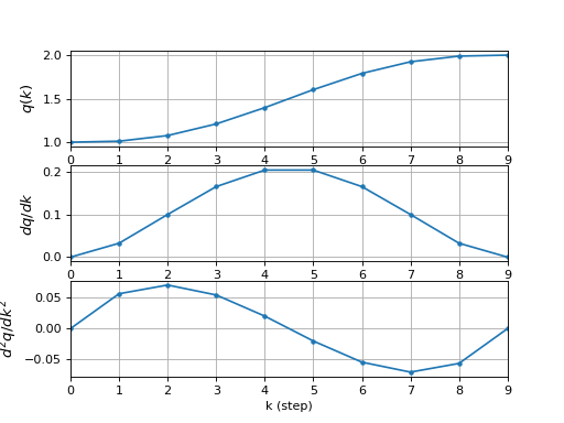
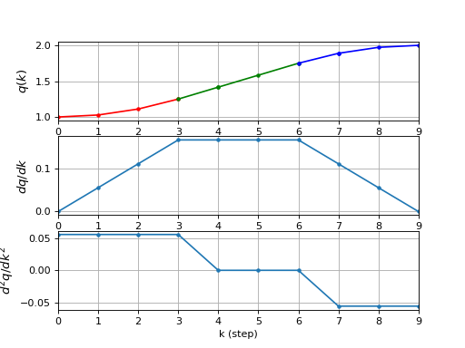
• quintic and trapezoidal show the individual points with markers

• trapezoidal color code the different motion phases

• jtraj general m-axis trajectory, show legend

Seealso:

quintic(), trapezoidal()

qplot(**kwargs)

Plot multi-axis trajectory

Parameters:

**kwargs –

optional arguments passed to qplot

Plots a multi-axis trajectory, held within the object, as position against time.

Seealso:

qplot()

roboticstoolbox.tools.trajectory.quintic(q0, qf, t, qd0=0, qdf=0)

Generate scalar polynomial trajectory

Parameters:

• q0 (float) – initial value

• qf (float) – final value

• t (int or array_like(m)) – time

• qd0 – initial velocity, optional

• qdf – final velocity, optional

Returns:

trajectory

Return type:

Trajectory instance

• tg = quintic(q0, q1, m) is a scalar trajectory (Mx1) that varies smoothly from q0 to qf using a quintic polynomial. The initial and final velocity and acceleration are zero. m is an integer scalar, indicating the total number of timesteps and

  • Velocity is in units of distance per trajectory step, not per second.

  • Acceleration is in units of distance per trajectory step squared, not per second squared.

• tg = quintic(q0, q1, t) as above but t is a uniformly-spaced time vector

  • Velocity is in units of distance per second.

  • Acceleration is in units of distance per second squared.

The return value is an object that contains position, velocity and acceleration data.

Example:

>>> from roboticstoolbox import quintic
>>> tg = quintic(1, 2, 10)
>>> tg
Trajectory created by quintic: 10 time steps x 1 axes
>>> len(tg)
10
>>> tg.q
array([1.    , 1.0115, 1.0764, 1.2099, 1.3967, 1.6033, 1.7901, 1.9236,
       1.9885, 2.    ])
>>> tg.plot()

(Source code, png, hires.png, pdf)

Note

The time vector T is assumed to be monotonically increasing, and time scaling is based on the first and last element.

References:

• Robotics, Vision & Control in Python, 3e, P. Corke, Springer 2023, Chap 3.

Seealso:

trapezoidal(), mtraj().

roboticstoolbox.tools.trajectory.quintic_func(q0, qf, T, qd0=0, qdf=0)

Quintic scalar polynomial as a function

Parameters:

• q0 (float, optional) – initial value

• qf (float) – final value

• T (float) – trajectory time

• qd0 – initial velocity, defaults to 0

• qdf – final velocity, defaults to 0

Returns:

polynomial function \(f: t \mapsto (q(t), \dot{q}(t), \ddot{q}(t))\)

Return type:

callable

Returns a function which computes the specific quintic polynomial, and its derivatives, as described by the parameters.

Example:

>>> from roboticstoolbox import quintic_func
>>> f = quintic_func(1, 2, 5)
>>> f(0)
(1.000000000000001, 2.782740400955608e-16, -8.565197162635485e-18)
>>> f(5)
(2.000000000000005, -3.233998897671231e-15, -7.225014857226153e-15)
>>> f(2.5)
(1.5000000000000029, 0.37500000000000167, 8.241020713062319e-16)

Seealso:

quintic() trapezoidal_func()

roboticstoolbox.tools.trajectory.lspb(*args, **kwargs)

Warning

Deprecated, use trapezoidal instead.

roboticstoolbox.tools.trajectory.trapezoidal(q0, qf, t, V=None)

Scalar trapezoidal trajectory

Parameters:

• q0 (float) – initial value

• qf (float) – final value

• t (float or array_like) – time

• V (float) – velocity of linear segment, optional

Returns:

trajectory

Return type:

Trajectory instance

Computes a trapezoidal trajectory, which has a linear motion segment with parabolic blends.

• tg = trapezoidal(q0, qf, t) is a scalar trajectory (Mx1) that varies smoothly from q0 to qf in M steps using a constant velocity segment and parabolic blends. Time t can be either:

  • an integer scalar, indicating the total number of timesteps

    • Velocity is in units of distance per trajectory step, not per second.

    • Acceleration is in units of distance per trajectory step squared, not per second squared.

  • an array_like, containing the time steps.

    • Results are scaled to units of time.

• tg = trapezoidal(q0, q1, t, V) as above but specifies the velocity of the linear segment which is normally computed automatically.

The return value is an object that contains position, velocity and acceleration data.

Example:

>>> from roboticstoolbox import trapezoidal
>>> tg = trapezoidal(1, 2, 10)
>>> tg
Trajectory created by trapezoidal: 10 time steps x 1 axes
>>> len(tg)
10
>>> tg.q
array([1.    , 1.0278, 1.1111, 1.25  , 1.4167, 1.5833, 1.75  , 1.8889,
       1.9722, 2.    ])

(Source code, png, hires.png, pdf)

Note

• For some values of V no solution is possible and an error is flagged.

• The time vector, if given, is assumed to be monotonically increasing, and time scaling is based on the first and last element.

• tg has an extra attribute xblend which is the blend duration.

References:

• Robotics, Vision & Control in Python, 3e, P. Corke, Springer 2023, Chap 3.

Seealso:

quintic(), trapezoidal_func() mtraj().

roboticstoolbox.tools.trajectory.trapezoidal_func(q0, qf, T, V=None)

Trapezoidal scalar profile as a function

Parameters:

• q0 (float) – initial value

• qf (float) – final value

• T (float) – maximum time

• V (float, optional) – velocity of linear segment

Returns:

trapezoidal profile function \(f: t \mapsto (q(t), \dot{q}(t), \ddot{q}(t))\)

Return type:

callable

Returns a function which computes the specific trapezoidal profile, and its derivatives, as described by the parameters.

Example:

>>> from roboticstoolbox import trapezoidal_func
>>> f = trapezoidal_func(1, 2, 5)
>>> f(0)
(array([1.]), array([0.]), array([0.18]))
>>> f(5)
(array([2.]), array([0.]), array([-0.18]))
>>> f(2.5)
(array([1.5]), array([0.3]), array([0]))

roboticstoolbox.tools.trajectory.mtraj(tfunc, q0, qf, t)

Multi-axis trajectory

Parameters:

• tfunc (callable) – a 1D trajectory function, eg. quintic() or trapezoidal()

• q0 (ndarray(m)) – initial configuration

• qf (ndarray(m)) – final configuration

• t (array_like or int) – time vector or number of steps

Raises:

• TypeError – tfunc is not callable

• ValueError – length of q0 and qf are different

Returns:

trajectory

Return type:

Trajectory instance

• tg = mtraj(func, q0, qf, n) is a multi-axis trajectory varying from configuration q0 (M) to qf (M) according to the scalar trajectory function tfunc in n steps.

• tg = mtraj(func, q0, qf, t) as above but t is a uniformly-spaced time vector

The scalar trajectory function is applied to each axis:

tg = tfunc(s0, sF, n)

and possible values of tfunc include trapezoidal for a trapezoidal trajectory, or quintic for a polynomial trajectory.

The return value is an object that contains position, velocity and acceleration data.

Note

The time vector, if given, is assumed to be monotonically increasing, and time scaling is based on the first and last element.

References:

• Robotics, Vision & Control in Python, 3e, P. Corke, Springer 2023, Chap 3.

Seealso:

quintic(), trapezoidal()

roboticstoolbox.tools.trajectory.jtraj(q0, qf, t, qd0=None, qd1=None)

Compute a joint-space trajectory

Parameters:

• q0 (array_like(n)) – initial joint coordinate

• qf (array_like(n)) – final joint coordinate

• t (array_like or int) – time vector or number of steps

• qd0 (array_like(n), optional) – initial velocity, defaults to zero

• qd1 (array_like(n), optional) – final velocity, defaults to zero

Returns:

trajectory

Return type:

Trajectory instance

• tg = jtraj(q0, qf, N) is a joint space trajectory where the joint coordinates vary from q0 (M) to qf (M). A quintic (5th order) polynomial is used with default zero boundary conditions for velocity and acceleration. Time is assumed to vary from 0 to 1 in N steps.

• tg = jtraj(q0, qf, t) as above but t is a uniformly-spaced time vector

The return value is an object that contains position, velocity and acceleration data.

Note

The time vector, if given, scales the velocity and acceleration outputs assuming that the time vector starts at zero and increases linearly.

References:

• Robotics, Vision & Control in Python, 3e, P. Corke, Springer 2023, Chap 3.

Seealso:

ctraj(), qplot(), jtraj()

roboticstoolbox.tools.trajectory.ctraj(T0, T1, t=None, s=None)

Cartesian trajectory between two poses

Parameters:

• T0 (SE3) – initial pose

• T1 (SE3) – final pose

• t (int or ndarray(n)) – number of samples or time vector

• s (ndarray(s)) – array of distance along the path, in the interval [0, 1]

Return T0:

smooth path from T0 to T1

Return type:

SE3

ctraj(T0, T1, n) is a Cartesian trajectory from SE3 pose T0 to T1 with n points that follow a trapezoidal velocity profile along the path. The Cartesian trajectory is an SE3 instance containing n values.

ctraj(T0, T1, t) as above but the trajectory is sampled at the points in the array t.

ctraj(T0, T1, s=s) as above but the elements of s specify the fractional distance along the path, and these values are in the range [0 1]. The i’th point corresponds to a distance s[i] along the path.

Examples:

>>> tg = ctraj(SE3.Rand(), SE3.Rand(), 20)
>>> len(tg)
20

Note

• In the second case s could be generated by a scalar trajectory

generator such as quintic or trapezoidal (default). - Orientation interpolation is performed using unit-quaternion interpolation.

References:

• Robotics, Vision & Control in Python, 3e, P. Corke, Springer 2023, Chap 3.

Seealso:

trapezoidal(), interp()

roboticstoolbox.tools.trajectory.cmstraj()

roboticstoolbox.tools.trajectory.mstraj(viapoints, dt, tacc, qdmax=None, tsegment=None, q0=None, qd0=None, qdf=None, verbose=False)

Multi-segment multi-axis trajectory

Parameters:

• viapoints (ndarray(m,n)) – A set of viapoints, one per row

• dt (float (seconds)) – time step

• tacc (float) – acceleration time (seconds)

• qdmax (array_like(n) or float, optional) – maximum speed, defaults to None

• tsegment (array_like, optional) – maximum time of each motion segment (seconds), defaults to None

• q0 (array_like(n), optional) – initial coordinates, defaults to first row of viapoints

• qd0 (array_like(n), optional) – inital velocity, defaults to zero

• qdf (array_like(n), optional) – final velocity, defaults to zero

• verbose (bool, optional) – print debug information, defaults to False

Returns:

trajectory

Return type:

Trajectory instance

Computes a trajectory for N axes moving smoothly through a set of viapoints. The motion comprises M segments:

• The initial coordinates are the first row of viapoints or q0 if provided.

• The final coordinates are the last row of viapoints

• Each segment is linear motion and polynomial blends connect the viapoints.

• All joints arrive at each via point at the same time, ie. the motion is coordinated across axes

The time of the segments can be specified in two different ways:

1. In terms of segment time where tsegment is an array of segment times which is the number of via points minus one:

   traj = mstraj(viapoints, dt, tacc, tsegment=TS)
   

2. Governed by the speed of the slowest axis for the segment. The axis speed is a scalar (all axes have the same speed) or an N-vector of speed per axis:

   traj = mstraj(viapoints, dt, tacc, qdmax=SPEED)
   

The return value is a namedtuple (named mstraj) with elements:

• t the time coordinate as a numpy ndarray, shape=(K,)

• q the axis values as a numpy ndarray, shape=(K,N)

• arrive a list of arrival times for each segment

• info a list of named tuples, one per segment that describe the slowest axis, segment time, and time stamp

• via the passed set of via points

The trajectory proper is (traj.t, traj.q). The trajectory is a matrix has one row per time step, and one column per axis.

Note

• Only one of qdmag or tsegment can be specified

• If tacc is greater than zero then the path smoothly accelerates between segments using a polynomial blend. This means that the the via point is not actually reached.

• The path length K is a function of the number of via points and the time or velocity limits that apply.

• Can be used to create joint space trajectories where each axis is a joint coordinate.

• Can be used to create Cartesian trajectories where the “axes” correspond to translation and orientation in RPY or Euler angle form.

• If qdmax is a scalar then all axes are assumed to have the same maximum speed.

• tg has extra attributes arrive, info and via

References:

• Robotics, Vision & Control in Python, 3e, P. Corke, Springer 2023, Chap 3.

Seealso:

trapezoidal(), ctraj(), mtraj()