Overview

Getting started

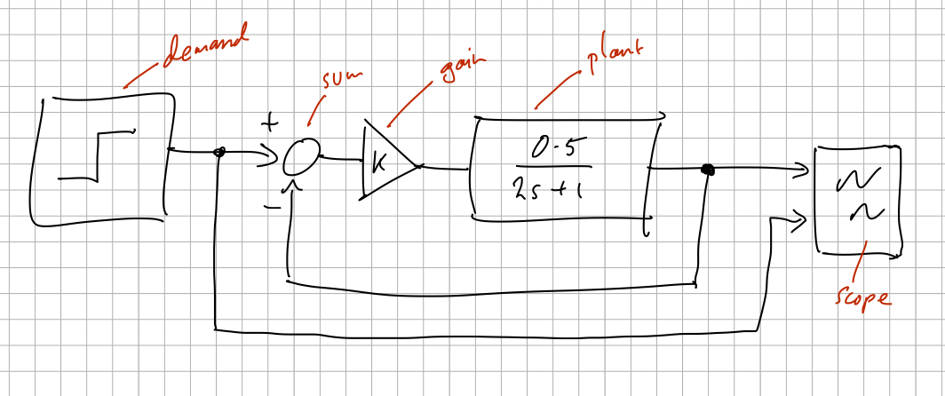
We first sketch the dynamic system we want to simulate as a block diagram, for example this simple first-order system:

which we can express concisely with bdsim as (see bdsim/examples/eg1.py):

import bdsim

sim = bdsim.BDSim()  # create simulator
bd = sim.blockdiagram()  # create an empty block diagram

# define the blocks
demand = bd.STEP(T=1, name='demand')
sum = bd.SUM('+-')
gain = bd.GAIN(10)
plant = bd.LTI_SISO(0.5, [2, 1], name='plant')
scope = bd.SCOPE(styles=['k', 'r--'], movie='eg1.mp4')

# connect the blocks
bd.connect(demand, sum[0], scope[1])
bd.connect(sum, gain)
bd.connect(gain, plant)
bd.connect(plant, sum[1], scope[0])

bd.compile()   # check the diagram
bd.report_summary()    # list all blocks and wires

out = sim.run(bd, 5)  # simulate for 5s

print(out)

This example utilizes just 16 lines of executable code. The red block annotations on the hand-drawn diagram correspond to the variable names holding references to the block instances.

Lines 7-11 defines the blocks used in the model. Blocks can have user-assigned names (see lines 7 and 10), which are useful for diagnostics and plot labels.
Lines 14-17 connects the blocks together. In bdsim, all wires are point-to-point, so a one-to-many connection is implemented by defining multiple wires. The first argument to connect is the source block, and subsequent arguments are destination blocks.
```
bd.connect(source, dest1, dest2, ...)
```
Ports are designated using Python indexing notation; for instance, block[2] refers to the third port of the block. Context determines if a port is an input or output: an index on the first argument of connect refers to an output, while subsequent arguments refer to inputs. If a block has only one port, the index 0 is assumed.

Groups of ports can be denoted using slice notation, for example:
```
bd.connect(source[2:5], dest[3:6])
```
connects source[2] to dest[3], source[3] to dest[4], and source[4] to dest[5].
Line 19 assembles the blocks, checks connectivity to create a flat wire list, and builds the dataflow execution plan.

Line 20 generates a tabular report summarizing the diagram’s blocks and wires.

┌─────────┬────┬────┬──────────┬────────┬────────┬─────────────┐
│  block  │ nc │ nd │   type   │ inport │ source │ source type │
├─────────┼────┼────┼──────────┼────────┼────────┼─────────────┤
│ demand@ │ 0  │ 0  │ step     │        │        │             │
├─────────┼────┼────┼──────────┼────────┼────────┼─────────────┤
│ gain.0  │ 0  │ 0  │ gain     │ 0      │ sum.0  │ float64     │
├─────────┼────┼────┼──────────┼────────┼────────┼─────────────┤
│ plant   │ 1  │ 0  │ lti_siso │ 0      │ gain.0 │ float64     │
├─────────┼────┼────┼──────────┼────────┼────────┼─────────────┤
│ scope.0 │ 0  │ 0  │ scope    │ 0      │ plant  │ float64     │
│         │    │    │          │ 1      │ demand │ int         │
├─────────┼────┼────┼──────────┼────────┼────────┼─────────────┤
│ sum.0   │ 0  │ 0  │ sum      │ 0      │ demand │ int         │
│         │    │    │          │ 1      │ plant  │ float64     │
└─────────┴────┴────┴──────────┴────────┴────────┴─────────────┘

Line 22 executes the simulation for the specified duration (5 seconds).
Line 26 (if uncommented) saves the scope content to a file named scope0.pdf.
Line 27 blocks the script execution until figure windows are closed or a SIGINT is received.

The simulation results are returned in a simple container object:

>>> print(out)
t      = ndarray:float64 (123,)
x      = ndarray:float64 (123, 1)
xnames = ['plant:x_0'] (list)

To record additional simulation variables, use a WATCH block or the watch option in run:

>>> out = sim.run(bd, 5, watch=[plant, demand])
>>> print(out)
t      = ndarray:float64 (123,)
x      = ndarray:float64 (123, 1)
xnames = ['plant:x_0'] (list)
y      = ndarray:float64 (123, 2)
ynames = ['demand', 'sum.0'] (list)
>>> plt.plot(out.t, out.y[:,0], 'k', out.t, out.y[:,1], 'r--')

Using operator overloading

Wiring and arithmetic blocks like GAIN, SUM, and PROD explicitly is somewhat tedious. An alternative is to implicitly generate and wire arithmetic blocks (GAIN, SUM, PROD) using overloaded Python operators, striking a balance between block diagram logic and Pythonic programming:

import bdsim

sim = bdsim.BDSim()
bd = sim.blockdiagram()

# define the blocks
demand = bd.STEP(T=1, name='demand')
plant = bd.LTI_SISO(0.5, [2, 1], name='plant')
scope = bd.SCOPE(styles=['k', 'r--'], movie='eg1.mp4')

# connect the blocks
scope[0] = plant
scope[1] = demand
plant[0] = 10 * (demand - plant)

bd.compile()
bd.report()

out = sim.run(bd, 5)
print(out)

sim.done(bd, block=True)

This approach requires fewer lines of code and is arguably is more readable, while producing exactly the same underlying block diagram. Implicitly created blocks are automatically named with an underscore prefix.

A list of available blocks can be obtained by:

>>> sim.blocks()
bdsim.blocks.connections................: ITEM DICT MUX DEMUX INDEX SUBSYSTEM INPORT OUTPORT
bdsim.blocks.continuous.................: INTEGRATOR POSEINTEGRATOR LTI_SS LTI_SISO DERIV2 DERIV PID
bdsim.blocks.displays...................: SCOPE SCOPEXY SCOPEXY1
bdsim.blocks.functions..................: SUM PROD GAIN POW CLIP FUNCTION INTERPOLATE
bdsim.blocks.linalg.....................: INVERSE TRANSPOSE NORM FLATTEN SLICE2 SLICE1 DET COND
bdsim.blocks.sampled....................: ZOH INTEGRATOR_S POSEINTEGRATOR_S DERIV_S LTI_SS_S LTI_SISO_S PID_S
........................................: DPOSEINTEGRATOR
bdsim.blocks.sinks......................: PRINT STOP EVENT NULL WATCH
bdsim.blocks.sources....................: CONSTANT TIME WAVEFORM PIECEWISE STEP RAMP
roboticstoolbox.blocks.arm..............: FKINE IKINE JACOBIAN ARMPLOT JTRAJ CTRAJ CIRCLEPATH TRAPEZOIDAL TRAJ IDYN
........................................: GRAVLOAD_X INERTIA INERTIA_X FDYN FDYN_X
roboticstoolbox.blocks.mobile...........: BICYCLE UNICYCLE DIFFSTEER VEHICLEPLOT
roboticstoolbox.blocks.spatial..........: TR2DELTA DELTA2TR POINT2TR TR2T
roboticstoolbox.blocks.uav..............: MULTIROTOR MULTIROTORMIXER MULTIROTORPLOT
machinevisiontoolbox.blocks.camera......: CAMERA VISJAC_P ESTPOSE_P IMAGEPLANE

More details can be found at: