Block library

The block diagrams comprise blocks which belong to one of a number of different categories. These come from the package bdsim.blocks, roboticstoolbox.blocks, machinevisiontoolbox.blocks.

Icons, if shown to the left of the black header bar, are as used with bdedit.

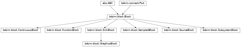
Block class hierarchy, arrow from parent class to subclass

Source blocks

Source blocks:

• have outputs but no inputs

• have no state variables

• are a subclass of SourceBlock → Block

class bdsim.blocks.sources.Constant(value=0, **blockargs)

Bases: SourceBlock

CONSTANT

Constant value.

Inputs:

0

Outputs:

1

States:

0

Port type	Port number	Types	Description
Output	0	any	constant value

The output value is a constant and can be any Python type, for example float, list or Numpy ndarray.

__init__(value=0, **blockargs)

Parameters:

• value (any, optional) – the constant, defaults to 0

• blockargs (dict) – common block options

class bdsim.blocks.sources.Piecewise(*args, seq=None, **blockargs)

Bases: SourceBlock, EventSource

PIECEWISE

Piecewise constant signal.

Inputs:

0

Outputs:

1

States:

0

Port type	Port number	Types	Description
Output	0	float	\(y(t)\)

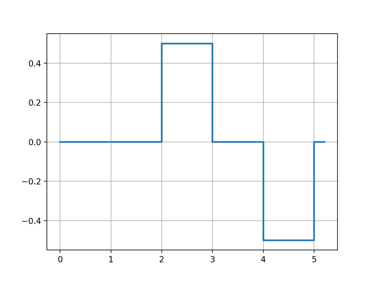
Generate a signal that is a piecewise constant function of time. This is described as a series of 2-tuples (time, value). The output value is taken from the active tuple, that is, the latest one in the list whose time is no greater than simulation time.

The tuples can be provided in two different ways. Firstly, a form convenient for Python programming:

steering = bd.PIECEWISE((0,0), (2, 0.5), (3,0), (4,-0.5), (5,0))

Secondly, in a form that can be used from bdsim where we explicitly pass in a list in a way that can be represented in a JSON file:

steering = bd.PIECEWISE(seq=[(0,0), (3, 0.5), (4,0), (5,-0.5), (6,0)])

(Source code, png, hires.png, pdf)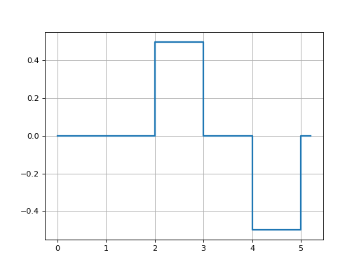

Note

• The tuples must be ordered by monotonically increasing time.

• There is no default initial value, the list should contain a tuple with time zero otherwise the output will be undefined.

Note

The block declares an event for the start of each segment.

Seealso:

declare_events()

__init__(*args, seq=None, **blockargs)

Parameters:

• seq (list of 2-element iterables) – sequence of time, value pairs

• blockargs (dict) – common block options

class bdsim.blocks.sources.Ramp(T=1, off=0, slope=1, **blockargs)

Bases: SourceBlock, EventSource

RAMP

Ramp signal.

Inputs:

0

Outputs:

1

States:

0

Port type	Port number	Types	Description
Output	0	float	\(y(t)\)

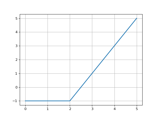
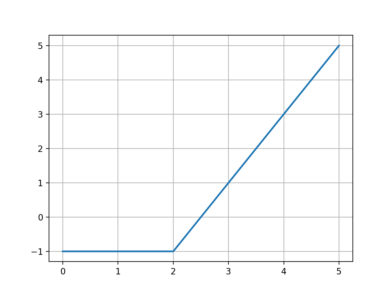
Generate a signal that starts increasing from the value off when time equals T linearly with time, with a gradient of slope.

Example:

step = bd.RAMP(2, off=-1, slope=2/3, T=2)

(Source code, png, hires.png, pdf)

Note

The block declares an event for the ramp start time.

Seealso:

declare_event()

__init__(T=1, off=0, slope=1, **blockargs)

Parameters:

• T (float, optional) – time of ramp start, defaults to 1

• off (float, optional) – initial value, defaults to 0

• slope (float, optional) – gradient of slope, defaults to 1

• blockargs (dict) – common block options

class bdsim.blocks.sources.Step(T=1, off=0, on=1, **blockargs)

Bases: SourceBlock, EventSource

STEP

Step signal.

Inputs:

0

Outputs:

1

States:

0

Port type	Port number	Types	Description
Output	0	float	\(y(t)\)

Generate a step signal that transitions from the value off to on when time equals T.

Example:

step = bd.STEP(2, off=-1, on=1)

(Source code, png, hires.png, pdf)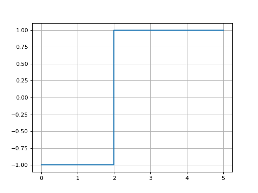

Note

The block declares an event for the step time.

Seealso:

declare_events()

__init__(T=1, off=0, on=1, **blockargs)

Parameters:

• T (float, optional) – time of step, defaults to 1

• off (float, optional) – initial value, defaults to 0

• on (float, optional) – final value, defaults to 1

• blockargs (dict) – common block options

class bdsim.blocks.sources.Time(value=None, **blockargs)

Bases: SourceBlock

TIME

Simulation time.

Inputs:

0

Outputs:

1

States:

0

Port type	Port number	Types	Description
Output	0	float	\(t\)

Outputs the current simulation time.

For example:

time = bd.TIME()

__init__(value=None, **blockargs)

Parameters:

blockargs (dict) – common block options

class bdsim.blocks.sources.WaveForm(wave='square', freq=1, unit='Hz', phase=0, amplitude=1, offset=0, min=None, max=None, duty=0.5, **blockargs)

Bases: SourceBlock, EventSource

WAVEFORM

Waveform generator.

Inputs:

0

Outputs:

1

States:

0

Port type	Port number	Types	Description
Output	0	float	\(y(t)\)

A general waveform generator. For example:

wave = bd.WAVEFORM(wave='sine', freq=2)   # 2Hz sine wave varying from -1 to 1
wave = bd.WAVEFORM(wave='square', freq=2, unit='rad/s') # 2rad/s square wave varying from -1 to 1

The minimum and maximum values of the waveform are given by default in terms of amplitude and offset. The signals are symmetric about the offset value. For example:

wave = bd.WAVEFORM(wave='sine') # varies between -1 and +1
wave = bd.WAVEFORM(wave='sine', amplitude=2) # varies between -2 and +2
wave = bd.WAVEFORM(wave='sine', offset=1) # varies between 0 and +2
wave = bd.WAVEFORM(wave='sine', amplitude=2, offset=1) # varies between -1 and +3

Alternatively we can specify the minimum and maximum values which override amplitude and offset:

wave = bd.WAVEFORM(wave='triangle', min=0, max=5) # varies between 0 and +5

At time 0 the sine and triangle wave are zero and increasing, and the square wave has its first rise. We can specify a phase shift with a number in the range [0,1] where 1 corresponds to one cycle.

Note

For discontinuous signals (square, triangle) the block declares events for every discontinuity.

Seealso:

declare_events()

__init__(wave='square', freq=1, unit='Hz', phase=0, amplitude=1, offset=0, min=None, max=None, duty=0.5, **blockargs)

Parameters:

• wave (str, optional) – type of waveform to generate, one of: ‘sine’, ‘square’ [default], ‘triangle’

• freq (float, optional) – frequency, defaults to 1

• unit (str, optional) – frequency unit, one of: ‘rad/s’, ‘Hz’ [default]

• amplitude (float, optional) – amplitude, defaults to 1

• offset (float, optional) – signal offset, defaults to 0

• phase (float, optional) – Initial phase of signal in the range [0,1], defaults to 0

• min (float, optional) – minimum value, defaults to None

• max (float, optional) – maximum value, defaults to None

• duty (float, optional) – duty cycle for square wave in range [0,1], defaults to 0.5

• blockargs (dict) – common block options

Sink blocks

Sink blocks:

• have inputs but no outputs

• have no state variables

• are a subclass of SinkBlock → Block

• that perform graphics are a subclass of GraphicsBlock → SinkBlock → Block

class bdsim.blocks.sinks.Event(direction, func, fargs=None, fkwargs=None, **blockargs)

Bases: SinkBlock

EVENT

Runtime event detector for solve_ivp.

Inputs:

1

Outputs:

0

States:

0

The input signal is used as an event function value. A zero crossing triggers an event in solve_ivp.

Direction can be one of:

• '^' or '+': positive-going crossing (direction = +1)

• 'v' or '-': negative-going crossing (direction = -1)

Event handling callback signature is:

func(block, *fargs, **fkwargs)

where block is this EVENT block instance.

__init__(direction, func, fargs=None, fkwargs=None, **blockargs)

Parameters:

• direction (str) – event crossing direction, one of '^', 'v', '+', '-'

• func (callable) – user callback invoked when event is detected

• fargs (list or tuple, optional) – extra positional args passed to callback

• fkwargs (dict, optional) – extra keyword args passed to callback

• blockargs (dict) – common block options

event_handler(t_crossing, y_crossing, state_map, simstate=None)

Return type:

None

class bdsim.blocks.sinks.Null(nin=1, **blockargs)

Bases: SinkBlock

NULL

Discard signal.

Inputs:

N

Outputs:

0

States:

0

Port type	Port number	Types	Description
Input	i	any	\(x_i\)

Create a sink block with arbitrary number of input ports that discards all data, like /dev/null. Useful for testing.

Note

bdsim issues a warning for unconnected outputs but execution can continue.

__init__(nin=1, **blockargs)

Parameters:

• nin (int, optional) – number of input ports, defaults to 1

• blockargs (dict) – common block options

class bdsim.blocks.sinks.Print(fmt=None, file=None, **blockargs)

Bases: SinkBlock

PRINT

Print signal.

Inputs:

1

Outputs:

0

States:

0

Port type	Port number	Types	Description
Input	0	any	\(x\)

Creates a console print block which displays the value of the input signal at each simulation time step. The display format is like:

PRINT(print.0 @ t=0.100) [-1.0 0.2]

and includes the block name, time, and the formatted value.

The numerical formatting of the signal is controlled by fmt:

• if not provided, str() is used to format the signal

• if provided:

  • a scalar is formatted by the fmt.format()

  • a NumPy array is formatted by fmt.format() applied to every element

Examples:

bd.PRINT(name="X")  # block name appears in the printed text
bd.PRINT(fmt="{:.1f}") # print with explicit format

Note

• By default writes to stdout

• The output is cleaner if progress bar printing is disabled using the -p command line option.

__init__(fmt=None, file=None, **blockargs)

Parameters:

• fmt (str, optional) – Format string, defaults to None

• file (file object, optional) – file to write data to, defaults to None

• blockargs (dict) – common block options

Returns:

A PRINT block

Return type:

Print instance

class bdsim.blocks.sinks.Stop(func=None, **blockargs)

Bases: SinkBlock

STOP

Conditionally stop simulation.

Inputs:

1

Outputs:

0

States:

0

Port type	Port number	Types	Description
Input	0	any	\(x\)

Conditionally stop the simulation if the input \(x\) is:

• bool type and True

• numeric type and > 0

If func is provided, then it is applied to the block input and if it returns True the simulation is stopped.

__init__(func=None, **blockargs)

Parameters:

• func (callable, optional) – evaluate stop condition, defaults to None

• blockargs (dict) – common block options

event_handler(t_crossing, y_crossing, state_map, simstate=None)

Return type:

None

class bdsim.blocks.sinks.Watch(nin=1, **blockargs)

Bases: SinkBlock

WATCH

Watch a signal.

Inputs:

N

Outputs:

0

States:

0

Port type	Port number	Types	Description
Input	i	any	\(x_i\)

Causes the output ports connected to this block’s input ports \(x_i\) to be logged during the simulation run. Equivalent to adding it as the watch= argument to bdsim.run.

For example:

step = bd.STEP(5)
ramp = bd.RAMP()
watch = bd.WATCH(2) # watch 2 ports
watch[0] = step
watch[1] = ramp

Seealso:

BDSim.run()

__init__(nin=1, **blockargs)

Parameters:

• nin (int, optional) – number of input ports, defaults to 1

• blockargs (dict) – common block options

Display blocks

Sink blocks:

• have inputs but no outputs

• have no state variables

• are a subclass of SinkBlock → Block

• that perform graphics are a subclass of GraphicsBlock → SinkBlock → Block

class bdsim.blocks.displays.Scope(nin=1, vector=None, styles=None, stairs=False, scale='auto', labels=None, grid=True, watch=False, title=None, loc='best', **blockargs)

Bases: GraphicsBlock

SCOPE

Plot input signals against time.

Inputs:

N

Outputs:

0

States:

0

Port type	Port number	Types	Description
Input	i	float	\(x_i\) is the i’th line

Create a scope block that plots multiple signals against time.

For each line plotted we can specify the:

• line style as a heterogeneous list of:

  • Matplotlib fmt string comprising a color and line style, eg. "k" or "r:"

  • a dict of Matplotlib line style options for Line2D , eg. {"color": "k", "linewidth": 3, "alpha": 0.5)

• line label, used in the legend and vertical axis. This can include math mode notation or unicode characters.

The vertical scale factor defaults to auto-scaling but can be fixed by providing a 2-tuple [ymin, ymax]. All lines are plotted against the same vertical scale.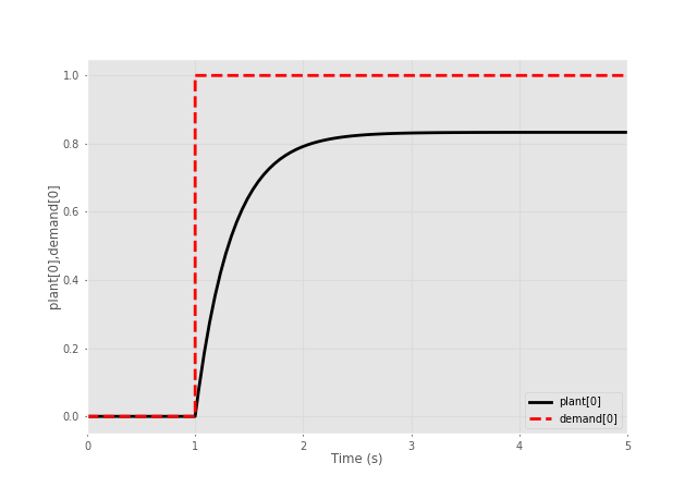

Example of scope display.

Scalar input ports against time

The number of lines to plot will be inferred from:

• the length of the labels list if specified

• the length of the styles list if specified

• nin if specified, it defaults to 1

These numbers must be consistent.

Examples:

bd.SCOPE()       # a scope with 1 input port
bd.SCOPE(nin=3)  # a scope with 3 input ports
bd.SCOPE(styles=["k", "r--"])        # a scope with 2 input ports
bd.SCOPE(labels=["x", r"$\gamma$"])  # a scope with 2 input ports
bd.SCOPE(styles=[{'color': 'blue'}, {'color': 'red', 'linestyle': '--'}])

Single input port with NumPy array

The port is fed with a 1D-array, and vector is an:

• int, this is the expected width of the array, all its elements will be plotted

• a list of ints, interpretted as indices of the elements to plot.

Examples:

bd.SCOPE(vector=[0,1,2]) # display elements 0, 1, 2 of array on port 0
bd.SCOPE(vector=[0,1], styles=[{'color': 'blue'}, {'color': 'red', 'linestyle': '--'}])

Note

• If the vector is of width 3, by default the inputs are plotted as red, green and blue lines.

• If the vector is of width 6, by default the first three inputs are plotted as solid red, green and blue lines and the last three inputs are plotted as dashed red, green and blue lines.

__init__(nin=1, vector=None, styles=None, stairs=False, scale='auto', labels=None, grid=True, watch=False, title=None, loc='best', **blockargs)

Parameters:

• nin (int, optional) – number of inputs, defaults to 1 or if given, the length of style vector

• vector (int or list, optional) – vector signal on single input port, defaults to None

• styles (str or dict, list of strings or dicts; one per line, optional) – styles for each line to be plotted

• stairs (bool, optional) – force staircase style plot for all lines, defaults to False

• scale (str or array_like(2)) – fixed y-axis scale or defaults to ‘auto’

• labels (sequence of strings) – labels for the plotted signals, defaults to block name and port of the source of each signal if not given. Used for vertical axis label, legend and cursor readout.

• grid (bool or sequence) – draw a grid, defaults to True. Can be boolean or a tuple of options for grid()

• watch (bool, optional) – add these signals to the watchlist, defaults to False

• title (str) – title of plot

• loc (str) – location of legend, see matplotlib.pyplot.legend(), defaults to “best”

• blockargs (dict) – common block options

class bdsim.blocks.displays.ScopeXY(style=None, scale='auto', aspect='equal', labels=['X', 'Y'], init=None, nin=2, **blockargs)

Bases: GraphicsBlock

SCOPEXY

Plot X against Y.

Inputs:

2

Outputs:

0

States:

0

Port type	Port number	Types	Description
Input	0	float	\(x\)
Input	1	float	\(y\)

Create an XY scope where input \(y\) (vertical axis) is plotted against \(x\) (horizontal axis).

Line style is one of:

• Matplotlib fmt string comprising a color and line style, eg. "k" or "r:"

• a dict of Matplotlib line style options for Line2D , eg. dict(color="k", linewidth=3, alpha=0.5)

The scale factor defaults to auto-scaling but can be fixed by providing either:

• a 2-tuple [min, max] which is used for the x- and y-axes

• a 4-tuple [xmin, xmax, ymin, ymax]

__init__(style=None, scale='auto', aspect='equal', labels=['X', 'Y'], init=None, nin=2, **blockargs)

Parameters:

• style (optional str or dict) – line style, defaults to None

• scale (str or array_like(2) or array_like(4)) – fixed y-axis scale or defaults to ‘auto’

• labels (2-element tuple or list) – axis labels (xlabel, ylabel), defaults to [“X”,”Y”]

• init (callable) – function to initialize the graphics, defaults to None

• blockargs (dict) – common block options

class bdsim.blocks.displays.ScopeXY1(indices=[0, 1], **blockargs)

Bases: ScopeXY

SCOPEXY1

Plot X[0] against X[1].

Inputs:

1

Outputs:

0

States:

0

Port type	Port number	Types	Description
Input	0	ndarray	\(x\)

Create an XY scope where input \(x_j\) (vertical axis) is plotted against \(x_i\) (horizontal axis). This block has one vector input and the elements to be plotted are given by a 2-element iterable \((i, j)\).

Line style is one of:

• Matplotlib fmt string comprising a color and line style, eg. "k" or "r:"

• a dict of Matplotlib line style options for Line2D , eg. dict(color="k", linewidth=3, alpha=0.5)

The scale factor defaults to auto-scaling but can be fixed by providing either:

• a 2-tuple [min, max] which is used for the x- and y-axes

• a 4-tuple [xmin, xmax, ymin, ymax]

__init__(indices=[0, 1], **blockargs)

Parameters:

• indices (array_like(2)) – indices of elements to select from block input vector, defaults to [0,1]

• style (optional str or dict) – line style

• scale (str or array_like(2) or array_like(4)) – fixed y-axis scale or defaults to ‘auto’

• labels (2-element tuple or list) – axis labels (xlabel, ylabel)

• init (callable) – function to initialize the graphics, defaults to None

• blockargs (dict) – common block options

Function blocks

Functions

Function blocks:

• have inputs and outputs

• have no state variables

• are a subclass of FunctionBlock → Block

class bdsim.blocks.functions.Clip(min=-inf, max=inf, **blockargs)

Bases: FunctionBlock

CLIP

Signal clipping.

Inputs:

1

Outputs:

1

States:

0

Port type	Port number	Types	Description
Input	0	int, float, ndarray	\(x\)
Output	0	int, float, ndarray	\(\min(\max(x,a), b)\)

The input signal is clipped to the range from minimum to maximum inclusive.

The signal can be a 1D-array in which case each element is clipped. The minimum and maximum values can be:

• a scalar, in which case the same value applies to every element of the input vector , or

• a 1D-array, of the same shape as the input vector that applies elementwise to the input vector.

For example:

clip = bd.CLIP(-1, 1)

__init__(min=-inf, max=inf, **blockargs)

Parameters:

• min (scalar or array_like, optional) – Minimum value, defaults to -math.inf

• max (float or array_like, optional) – Maximum value, defaults to math.inf

• blockargs (dict) – common block options

class bdsim.blocks.functions.Function(func=None, nin=1, nout=1, persistent=False, fargs=None, fkwargs=None, **blockargs)

Bases: FunctionBlock

FUNCTION

Python function.

Inputs:

N

Outputs:

M

States:

0

Port type	Port number	Types	Description
Input	i	any	\(x_i\)
Output	j	any	\(f_j(x_0, \ldots, x_{N-1})\)

Inputs to the block are passed as separate arguments to the function. Programmatic ositional or keyword arguments can also be passed to the function.

A block with one output port that sums its two input ports is:

func = bd.FUNCTION(lambda u1, u2: u1+u2, nin=2)

A block with a function that takes two inputs and has two additional arguments:

def myfun(u1, u2, param1, param2):
    pass

FUNCTION(myfun, nin=2, args=(p1,p2))

If we need access to persistent (static) data, to keep some state:

def myfun(u1, u2, param1, param2, state):
    pass

func = bd.FUNCTION(myfun, nin=2, args=(p1,p2), persistent=True)

where a dictionary is passed in as the last argument and which is kept from call to call.

A block with a function that takes two inputs and additional keyword arguments:

def myfun(u1, u2, param1=1, param2=2, param3=3, param4=4):
    pass

func = bd.FUNCTION(myfun, nin=2, kwargs=dict(param2=7, param3=8))

A block with two inputs and two outputs, the outputs are defined by two lambda functions with the same inputs:

FUNCTION( [ lambda x, y: x_t, lambda x, y: x* y])

A block with two inputs and two outputs, the outputs are defined by a single function which returns a list:

def myfun(u1, u2):
    return [ u1+u2, u1*u2 ]

func = bd.FUNCTION( myfun, nin=2, nout=2)

__init__(func=None, nin=1, nout=1, persistent=False, fargs=None, fkwargs=None, **blockargs)

Parameters:

• func (callable or sequence of callables, optional) – function or lambda, or list thereof, defaults to None

• nin (int, optional) – number of inputs, defaults to 1

• nout (int, optional) – number of outputs, defaults to 1

• persistent (bool, optional) – pass in a reference to a dictionary instance to hold persistent state, defaults to False

• fargs (list, optional) – extra positional arguments passed to the function, defaults to []

• fkwargs (dict, optional) – extra keyword arguments passed to the function, defaults to {}

• blockargs (dict, optional) – common block options

class bdsim.blocks.functions.Gain(K=1, premul=False, **blockargs)

Bases: FunctionBlock

GAIN

Gain block.

Inputs:

1

Outputs:

1

States:

0

Port type	Port number	Types	Description
Input	0	int, float, ndarray	\(x\)
Output	0	int, float, ndarray	\(K x\)

Either or both the input and gain can be Numpy arrays and Numpy will compute the appropriate product \(u K\).

If \(u\) and K are both NumPy arrays the @ operator is used and \(u\) is postmultiplied by the gain. To premultiply by the gain, to compute \(K u\) use the premul option.

For example:

gain = bd.GAIN(2.5)

__init__(K=1, premul=False, **blockargs)

Parameters:

• K (scalar, array_like) – The gain value, defaults to 1

• premul (bool, optional) – premultiply by constant, default is postmultiply, defaults to False

• blockargs (dict) – common block options

class bdsim.blocks.functions.Interpolate(x=None, y=None, xy=None, time=False, kind='linear', **blockargs)

Bases: FunctionBlock

INTERPOLATE

Interpolate signal.

Inputs:

1

Outputs:

1

States:

0

Port type	Port number	Types	Description
Input	0	int, float	\(x\)
Output	0	float	\(f(x)\)

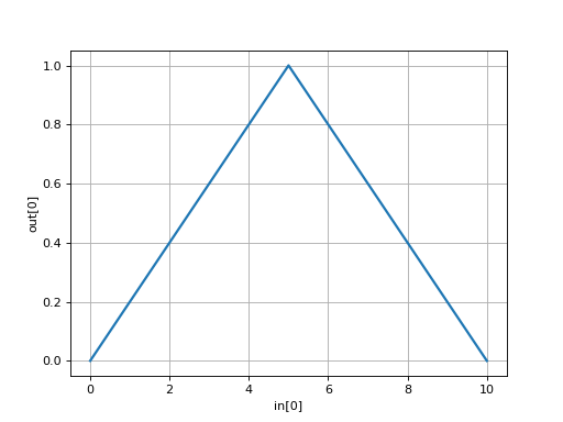
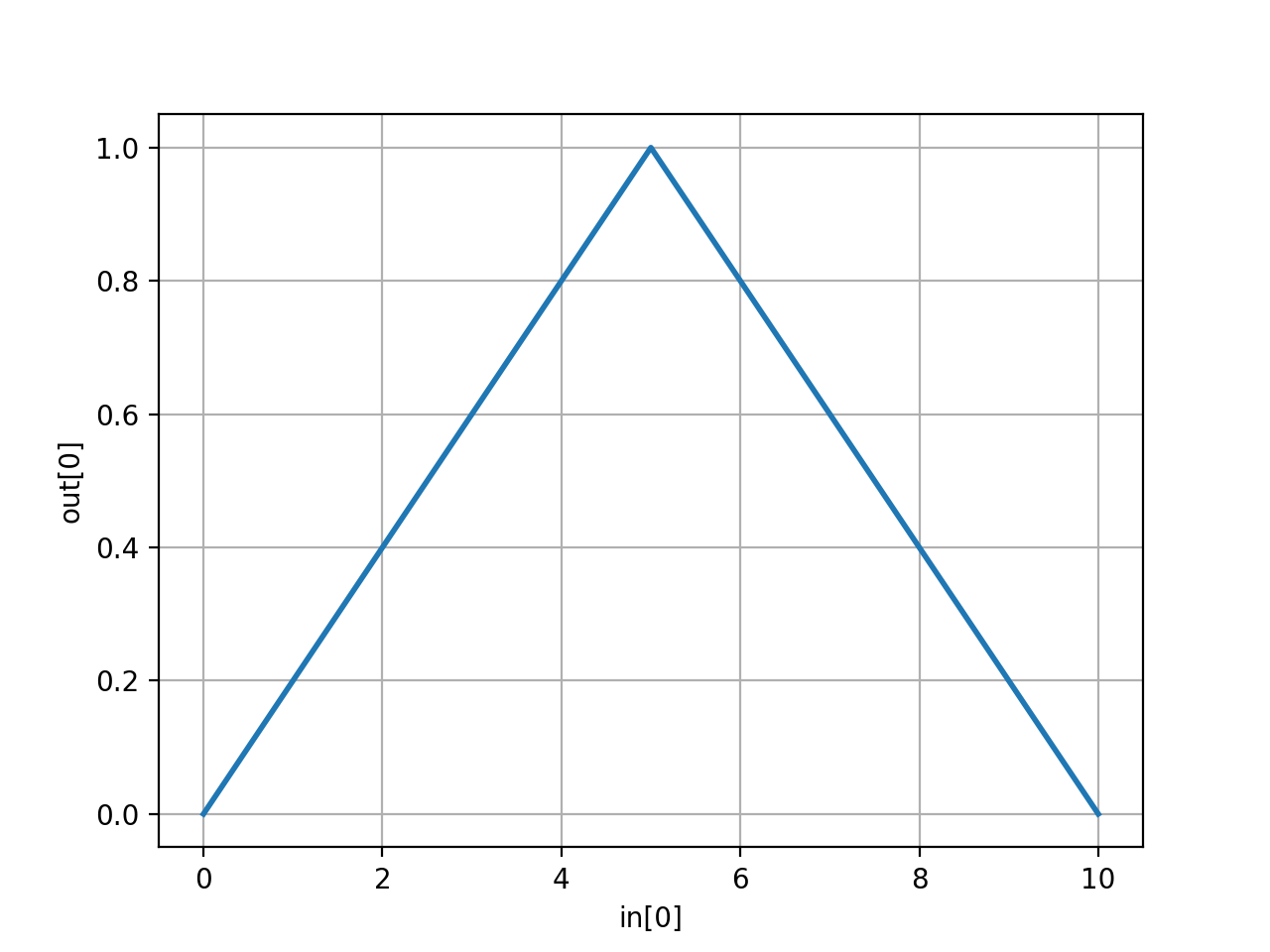
Interpolate a scalar function of a scalar.

A simple triangle function with domain [0,10] and range [0,1] can be defined by:

interp = bd.INTERPOLATE(x=(0,5,10), y=(0,1,0))

We might also express this as a list of 2D-coordinates:

interp = bd.INTERPOLATE(xy=[(0,0), (5,1), (10,0)])

(Source code, png, hires.png, pdf)

The data can also be expressed as Numpy arrays. If that is the case, the interpolation function can be vector valued. x has a shape of (N,1) and y has a shape of (N,M). Alternatively xy has a shape of (N,M+1) and the first column is the x-data.

Note:

if time=True then the block has no input ports and acts as a Source not a Function block.

Seealso:

scipy.interpolate.interp1d()

__init__(x=None, y=None, xy=None, time=False, kind='linear', **blockargs)

Parameters:

• x (array_like, shape (N,) optional) – x-values of function, defaults to None

• y (array_like, optional) – y-values of function, defaults to None

• xy (array_like, optional) – combined x- and y-values of function, defaults to None

• time (bool, optional) – x new is simulation time, defaults to False

• kind (str, optional) – interpolation method, defaults to ‘linear’

• blockargs (dict) – common block options

class bdsim.blocks.functions.Pow(p=1, matrix=False, **blockargs)

Bases: FunctionBlock

POW

Power block.

Inputs:

1

Outputs:

1

States:

0

Port type	Port number	Types	Description
Input	0	int, float, ndarray	\(x\)
Output	0	int, float, ndarray	\(x^p\)

If the input is a Numpy array the result depends on matrix. If matrix is False the block performs an elementwise exponentiation and the result is a Numpy array of the same size.

If matrix is True and the input is a square matrix and p is an integer then matrixwise exponentiation is performedand using repeated matrix multiplication and matrix inversion. If p is not an integer it uses SciPy to compute the power using an eigenvalue decomposition.

For example:

pow = bd.POW(2)

Seealso:

numpy.linalg.matrix_power() scipy.linalg.fractional_matrix_power()

__init__(p=1, matrix=False, **blockargs)

Parameters:

• p (scalar) – The exponent value, defaults to 1

• matrix (bool, optional) – premultiply by constant, default is postmultiply, defaults to False

• blockargs (dict) – common block options

class bdsim.blocks.functions.Prod(ops='**', matrix=False, **blockargs)

Bases: FunctionBlock

PROD

Product junction.

Inputs:

N

Outputs:

1

States:

0

Port type	Port number	Types	Description
Input	i	int, float, ndarray	\(x_i\)
Output	0	int, float, ndarray	\(\prod_i \{x_i | \frac{1}{x_i}\}\)

Multiply or divide input signals according to the ops string. The number of input ports is the length of this string.

For example:

prod = PROD('*/*')

is a 3-input product junction which computes in[0] / in[1] * in[2].

Note:

By default the * and / operators are used which perform element-wise operations.

Note:

The option matrix will instead use @ and @ np.linalg.inv(). The shapes of matrices must conform. A matrix on a / input must be square and non-singular. Matrices are multiplied in ascending port order.

__init__(ops='**', matrix=False, **blockargs)

Parameters:

• ops (str, optional) – operations associated with input ports, accepted characters: * or /, defaults to ‘**’

• inputs (Block or Plug) – Optional incoming connections

• matrix (bool, optional) – Arguments are matrices, defaults to False

• blockargs (dict) – common block options

class bdsim.blocks.functions.Sum(signs='++', mode=None, **blockargs)

Bases: FunctionBlock

SUM

Summing junction.

Inputs:

N

Outputs:

1

States:

0

Port type	Port number	Types	Description
Input	i	int, float, ndarray	\(x_i\)
Output	0	int, float, ndarray	\(\sum_i \pm x_i\)

Add or subtract input signals according to the signs string. The number of input ports is the length of this string.

For example:

sum = bd.SUM('+-+')

is a 3-input summing junction which computes in[0] - in[1] + in[2].

Note:

The signals must be compatible for addition, and if some are arrays they must be broadcastable.

__init__(signs='++', mode=None, **blockargs)

Parameters:

• signs (str, optional) – a string comprising + or - characters, defaults to ++

• mode (str, optional) – controls addition mode, per element, string comprises r or c or C or L, defaults to None

• blockargs (dict) – common block options

For example the string +- creates a 2-port block where the second input is subtracted from the first.

mode controls how elements of the input vectors are added/subtracted. Elements which are angles must be treated specially, and this is indicated by the corresponding characters in mode. The string’s length must equal the width of the input vectors. The characters of the string can be:

mode character	purpose
r	real number, don’t wrap (default)
c	angle on circle, wrap to [-π, π)
C	angle on circle, wrap to [0, 2π)
L	colatitude angle, wrap to [0, π]

For example if mode="rc" then a 2-element array would have its second element wrapped to the range [-π, π).

Linear algebra

Linear algebra blocks:

• have inputs and outputs

• have no state variables

• are a subclass of FunctionBlock → Block

class bdsim.blocks.linalg.Cond(**blockargs)

Bases: FunctionBlock

COND

Matrix condition number.

Inputs:

1

Outputs:

1

States:

0

Port type	Port number	Types	Description
Input	0	ndarray	\(\mathbf{A}\)
Output	0	ndarray	\(\mbox{cond}(\mathbf{A})\)

Seealso:

numpy.linalg.cond()

__init__(**blockargs)

Parameters:

blockargs (dict) – common block options

class bdsim.blocks.linalg.Det(**blockargs)

Bases: FunctionBlock

DET

Matrix determinant.

Inputs:

1

Outputs:

1

States:

0

Port type	Port number	Types	Description
Input	0	ndarray	\(\mathbf{A}\)
Output	0	ndarray	\(\mbox{det}(\mathbf{A})\)

Compute the matrix determinant.

Seealso:

numpy.linalg.det()

__init__(**blockargs)

Parameters:

blockargs (dict) – common block options

class bdsim.blocks.linalg.Flatten(order='C', **blockargs)

Bases: FunctionBlock

FLATTEN

Flatten a multi-dimensional array.

Inputs:

1

Outputs:

1

States:

0

Port type	Port number	Types	Description
Input	0	ndarray	\(\mathbf{A}\)
Output	0	ndarray	\(\mbox{vec}(\mathbf{A})\)

Flattens the incoming array in either row major (‘C’) or column major (‘F’) order.

Seealso:

numpy.ndarray.flatten()

__init__(order='C', **blockargs)

Parameters:

• order (str) – flattening order, either “C” or “F”, defaults to “C”

• blockargs (dict) – common block options

class bdsim.blocks.linalg.Inverse(pinv=False, **blockargs)

Bases: FunctionBlock

INVERSE

Matrix inverse.

Inputs:

1

Outputs:

2

States:

0

Port type	Port number	Types	Description
Input	0	ndarray	\(\mathbf{A}\)
Output	0	ndarray	\(\mathbf{A}^{-1}\)
Output	1	float	\(\mbox{cond}(\mathbf{A})\)

Compute inverse of the 2D-array input signal. If the matrix is square the inverse is computed unless the pinv flag is True. For a non-square matrix the pseudo-inverse is used. The condition number is output on the second port.

Seealso:

numpy.linalg.inv() numpy.linalg.pinv() numpy.linalg.cond()

__init__(pinv=False, **blockargs)

Parameters:

• pinv (bool, optional) – force pseudo inverse, defaults to False

• blockargs (dict) – common block options

onames = ('inv', 'cond')

class bdsim.blocks.linalg.Norm(ord=None, axis=None, **blockargs)

Bases: FunctionBlock

NORM

Array norm.

Inputs:

1

Outputs:

1

States:

0

Port type	Port number	Types	Description
Input	0	ndarray	\(\mathbf{A}\)
Output	0	ndarray	\(\|\mathbf{A}\|\)

Computes the specified norm for a 1D- or 2D-array.

Seealso:

numpy.linalg.norm()

__init__(ord=None, axis=None, **blockargs)

Parameters:

• axis (int, optional) – specifies the axis along which to compute the vector norms, defaults to None.

• ord (int or str) – Order of the norm, default to None.

• blockargs (dict) – common block options

class bdsim.blocks.linalg.Slice1(index, **blockargs)

Bases: FunctionBlock

SLICE1

Slice out subarray of 1D-array.

Inputs:

1

Outputs:

1

States:

0

Port type	Port number	Types	Description
Input	0	ndarray	\(v\)
Output	0	ndarray	\(v_{i\dots j}\)

Compute a 1D slice of input 1D array.

If index is None it means all elements.

If index is a list, perform NumPy fancy indexing, returning the specified elements

Example:

slice = bd.SLICE1(index=[2,3]) # return elements 2 and 3 as a 1D array
slice = bd.SLICE1(index=[2])   # return element 2 as a 1D array
slice = bd.SLICE1(index=2)     # return element 2 as a NumPy scalar

If index is a tuple, it must have three elements. It describes a Python slice (start, stop, step) where any element can be None

• start=None means start at first element

• stop=None means finish at last element

• step=None means step by one

rows=None is equivalent to rows=(None, None, None).

Example:

slice = bd.SLICE1(index=(None,None,2))  # return every second element
slice = bd.SLICE1(index=(None,None,-1)) # reverse the elements

Seealso:

Slice1

__init__(index, **blockargs)

Parameters:

• index (tuple(3)) – slice, defaults to None

• blockargs (dict) – common block options

class bdsim.blocks.linalg.Slice2(rows=None, cols=None, **blockargs)

Bases: FunctionBlock

SLICE2

Slice out subarray of 2D-array.

Inputs:

1

Outputs:

1

States:

0

Port type	Port number	Types	Description
Input	0	ndarray	\(\mathbf{A}\)
Output	0	ndarray	\(\mathbf{A}_{i\ldots j, m\ldots n}\)

Compute a 2D slice of input 2D array.

If rows or cols is None it means all rows or columns respectively.

If rows or cols is a list, perform NumPy fancy indexing, returning the specified rows or columns

Example:

slice = bd.SLICE2(rows=[2,3])  # return rows 2 and 3, all columns
slice = bd.SLICE2(cols=[4,1])  # return columns 4 and 1, all rows
slice = bd.SLICE2(rows=[2,3], cols=[4,1]) # return elements [2,4] and [3,1] as a 1D array

If a single row or column is selected, the result will be a 1D array

If rows or cols is a tuple, it must have three elements. It describes a Python slice (start, stop, step) where any element can be None

• start=None means start at first element

• stop=None means finish at last element

• step=None means step by one

rows=None is equivalent to rows=(None, None, None).

Example:

slice = bd.SLICE2(rows=(None,None,2))  # return every second row
slice = bd.SLICE2(cols=(None,None,-1)) # reverse the columns

The list and tuple notation can be mixed, for example, one for rows and one for columns.

Seealso:

Slice1 Index

__init__(rows=None, cols=None, **blockargs)

Parameters:

• rows (tuple(3) or list) – row selection, defaults to None

• cols (tuple(3) or list) – column selection, defaults to None

• blockargs (dict) – common block options

class bdsim.blocks.linalg.Transpose(**blockargs)

Bases: FunctionBlock

TRANSPOSE

Matrix transpose.

Inputs:

1

Outputs:

2

States:

0

Port type	Port number	Types	Description
Input	0	ndarray	\(\mathbf{A}\)
Output	0	ndarray	\(\mathbf{A}^{\top}\)

Compute transpose of the 2D-array input signal.

Note

• An input 1D-array of shape (N,) is turned into a 2D-array column vector with shape (N,1).

• An input 2D-array column vector of shape (N,1) becomes a 2D-array row vector with shape (1,N).

Seealso:

numpy.linalg.transpose()

__init__(**blockargs)

Parameters:

blockargs (dict) – common block options

Spatial math

class bdsim.blocks.spatial.Pose_inverse(**blockargs)

Bases: FunctionBlock

POSE_INVERSE

Pose inverse.

Inputs:

1

Outputs:

1

States:

0

Port type	Port number	Types	Description
Input	0	SEn, SOn	\(\xi\)
Output	0	SEn, SOn	\(\ominus \xi\)

Invert the pose on the input port.

__init__(**blockargs)

Parameters:

blockargs (dict) – common block options

class bdsim.blocks.spatial.Pose_postmul(pose=None, **blockargs)

Bases: FunctionBlock

POSE_POSTMUL

Post multiply pose.

Inputs:

1

Outputs:

1

States:

0

Port type	Port number	Types	Description
Input	0	SEn, SOn	\(\xi\)
Output	0	SEn, SOn	\(\xi \oplus \xi_c\)

Postmultiply the input pose by a constant pose.

Note

Pose objects must be of the same type.

Seealso:

Pose_premul

__init__(pose=None, **blockargs)

Parameters:

• pose (SO2, SE2, SO3 or SE3) – pose to apply

• blockargs (dict) – common block options

class bdsim.blocks.spatial.Pose_premul(pose=None, **blockargs)

Bases: FunctionBlock

POSE_PREMUL

Pre multiply pose.

Inputs:

1

Outputs:

1

States:

0

Port type	Port number	Types	Description
Input	0	SEn, SOn	\(\xi\)
Output	0	SEn, SOn	\(\xi_c \oplus \xi\)

Premultiply the input pose by a constant pose.

Note

Pose objects must be of the same type.

Seealso:

Pose_postmul

__init__(pose=None, **blockargs)

Parameters:

• pose (SO2, SE2, SO3 or SE3) – pose to apply

• blockargs (dict) – common block options

class bdsim.blocks.spatial.Transform_vector(**blockargs)

Bases: FunctionBlock

TRANSFORM_VECTOR

Transform a vector.

Inputs:

2

Outputs:

1

States:

0

Port type	Port number	Types	Description
Input	0	SEn, SOn	\(\xi\)
Input	1	ndarray	\(v\), Euclidean 2D or 3D
Output	0	ndarray	\(\xi \bullet v\)

Linearly transform the input vector by the input pose.

__init__(**blockargs)

Parameters:

blockargs (dict) – common block options

Connection blocks

Connection blocks are in two categories:

1. Signal manipulation:

   • have inputs and outputs

   • have no state variables

   • are a subclass of FunctionBlock → Block

2. Subsystem support

   • have inputs or outputs

   • have no state variables

   • are a subclass of SubsysytemBlock → Block

class bdsim.blocks.connections.DeMux(nout=1, **blockargs)

Bases: FunctionBlock

DEMUX

Demultiplex signals.

Inputs:

1

Outputs:

N

States:

0

Port type	Port number	Types	Description
Input	0	iterable	\(x\)
Output	i	any	\(x_i\)

This block has a single input port and nout output ports. The input signal is an iterable whose nout elements are routed element-wise to individual scalar output ports. If the input is a 1D Numpy array, then each output port is an element of that array.

Seealso:

Mux

__init__(nout=1, **blockargs)

Parameters:

• nout (int, optional) – number of outputs, defaults to 1

• blockargs (dict) – common block options

class bdsim.blocks.connections.Dict(keys, **blockargs)

Bases: FunctionBlock

DICT

Create a dictionary signal.

Inputs:

N

Outputs:

1

States:

0

Port type	Port number	Types	Description
Input	i	any	\(x_i\)
Output	0	dict	{key: x[i] for i, key in enumerate(keys)}

Inputs are assigned to a dictionary signal, using the corresponding names from keys. For example:

dd = bd.DICT(["x", "xd", "xdd"])

expects three inputs and assigns them to dictionary items x, xd, xdd of the output dictionary respectively.

This is somewhat like a multiplexer Mux but allows for named heterogeneous data. A dictionary signal can serve a similar purpose to a “bus” in Simulink(R).

Seealso:

Item Mux

__init__(keys, **blockargs)

Parameters:

• keys (list) – list of dictionary keys

• blockargs (dict) – common block options

class bdsim.blocks.connections.InPort(nout=1, **blockargs)

Bases: FunctionBlock

INPORT

Input ports for a subsystem.

Inputs:

0

Outputs:

N

States:

0

Port type	Port number	Types	Description
Output	j	any	\(y_j\)

This block connects a subsystem to a parent block diagram. Inputs to the parent-level SubSystem block appear as the outputs of this block.

Note

Only one INPORT block can appear in a block diagram but it can have multiple ports. This is different to Simulink(R) which would require multiple single-port input blocks.

__init__(nout=1, **blockargs)

Parameters:

• nout (int, optional) – Number of output ports, defaults to 1

• blockargs (dict) – common block options

class bdsim.blocks.connections.Index(index=None, **blockargs)

Bases: FunctionBlock

INDEX

Inputs:

1

Outputs:

1

States:

0

Port type	Port number	Types	Description
Input	i	iterable	\(x\)
Output	j	iterable	\(x_i\)

The specified element(s) of the input iterable (list, string, etc.) are output. The index can be an integer, sequence of integers, a Python slice object, or a string with Python slice notation, eg. "::-1".

Seealso:

Slice1 Slice2

__init__(index=None, **blockargs)

Index an iterable signal.

Parameters:

• index (list, slice or str, optional) – elements of input array, defaults to []

• blockargs (dict) – common block options

class bdsim.blocks.connections.Item(item, **blockargs)

Bases: FunctionBlock

ITEM

Select item from a dictionary signal.

Inputs:

1

Outputs:

1

States:

0

Port type	Port number	Types	Description
Input	0	dict	D
Output	0	any	D[i]

For a dictionary type input signal, select one item as the output signal. For example:

item = bd.ITEM("xd")

selects the xd item from the dictionary signal input to the block.

This is somewhat like a demultiplexer DeMux but allows for named heterogeneous data. A dictionary signal can serve a similar purpose to a “bus” in Simulink(R).

Seealso:

Dict

__init__(item, **blockargs)

Parameters:

• item (str) – name of dictionary item

• blockargs (dict) – common block options

class bdsim.blocks.connections.Mux(nin=1, **blockargs)

Bases: FunctionBlock

MUX

Multiplex signals.

Inputs:

N

Outputs:

1

States:

0

Port type	Port number	Types	Description
Input	i	float, ndarray	\(x_i\)
Output	0	ndarray	\([x_0 \ldots x_{N-1}]\)

This block takes a number of scalar or 1D-array signals and concatenates them into a single 1-D array signal. For example:

mux = bd.MUX(2)

Seealso:

Demux Dict

__init__(nin=1, **blockargs)

Parameters:

• nin (int, optional) – Number of input ports, defaults to 1

• blockargs (dict) – common block options

class bdsim.blocks.connections.OutPort(nin=1, **blockargs)

Bases: FunctionBlock

OUTPORT

Output ports for a subsystem.

Inputs:

N

Outputs:

0

States:

0

Port type	Port number	Types	Description
Input	i	any	\(x_i\)

This block connects a subsystem to a parent block diagram. The inputs of this block become the outputs of the parent-level SubSystem block.

Note

Only one OUTPORT block can appear in a block diagram but it can have multiple ports. This is different to Simulink(R) which would require multiple single-port output blocks.

__init__(nin=1, **blockargs)

Parameters:

• nin (int, optional) – Number of input ports, defaults to 1

• blockargs (dict) – common block options

class bdsim.blocks.connections.SubSystem(subsys, nin=1, nout=1, allow_eval=None, trace_eval=False, globalvars=None, **blockargs)

Bases: SubsystemBlock

SUBSYSTEM

Instantiate a subsystem.

Inputs:

N

Outputs:

M

States:

0

Port type	Port number	Types	Description
Input	i	any	\(x_i\)
Output	j	any	\(y_j\)

This block represents a subsystem in a block diagram. The definition of the subsystem can be:

• a path to a .bd JSON model file, which is loaded via bdload(), or

• the name of a Python module which is imported and must create exactly one BlockDiagram instance, or

• a BlockDiagram instance

Warning

Module name mode (non-.bd string): importing a module executes all top-level Python code in that file. Only use this with modules you trust completely.

File mode (.bd path): loads a JSON file safely. eval() is only used for parameters starting with "="; control this with allow_eval.

The referenced block diagram must contain either or both of:

• one InPort block, which has outputs but no inputs. These outputs are connected to the inputs to the enclosing SubSystem block.

• one OutPort block, which has inputs but no outputs. These inputs are connected to the outputs to the enclosing SubSystem block.

Note

• The referenced block diagram is treated like a macro and copied into the parent block diagram at compile time. The SubSystem, InPort and OutPort blocks are eliminated, that is, all hierarchical structure is lost.

• The same subsystem can be used multiple times, its blocks and wires will be cloned. Subsystems can also include subsystems.

• The number of input and output ports is not specified, they are computed from the number of ports on the InPort and OutPort blocks within the subsystem.

__init__(subsys, nin=1, nout=1, allow_eval=None, trace_eval=False, globalvars=None, **blockargs)

Parameters:

• subsys (str or BlockDiagram) – Subsystem as a .bd filepath, module name, or BlockDiagram instance

• nin (int, optional) – Number of input ports, defaults to 1

• nout (int, optional) – Number of output ports, defaults to 1

• allow_eval (bool, optional) – (.bd mode only) True enables eval silently, False refuses =... expressions, None (default) warns once.

• trace_eval (bool, optional) – (.bd mode only) print each expression before evaluation.

• globalvars (dict, optional) – (.bd mode only) extra names available when evaluating "=..." parameter expressions.

• blockargs (dict) – common block options

Raises:

• ImportError – module not found or no BlockDiagram in it

• ValueError – invalid argument type or .bd load constraints not met

Continuous-time dynamics

Continuous-time blocks:

• have inputs and outputs

• have state variables

• are a subclass of ContinuousBlock → Block

class bdsim.blocks.continuous.Deriv(alpha, x0=0, y0=None, gain=1.0, **blockargs)

Bases: SubsystemBlock

DERIV

Continuous-time derivative.

Inputs:

1

Outputs:

1

States:

N

Port type	Port number	Types	Description
Input	0	float	\(x\)
Output	0	float	\(y\)

Implements the dynamics of a derivative filter, but to be causal (proper) it includes a first-order low-pass filter. The dynamics is

\[\frac{s}{\frac{s}{\alpha} + 1}\]

The pole is at \(s=-\alpha\). A small value of alpha corresponds to a long-time constant in the step reponse. The parameter alpha can be used to achieve the desired tradeoff between noise reduction and phase lag.

The derivative calculation is performed using a complementary filter, implemented as a subsystem with an integrator and a feedback loop. The initial state of the integrator is given by x0:

    +
u ───> SUM ───────> GAIN(alpha) ──┬───>  GAIN(k) ───> y
        ▲ ─                       │
        │                         │
        └───  INTEGRATOR(x0) <────┘

If the initial output of the derivative block is known it can be provided as y0 from which x0 is calculated by \(x_0 = - \alpha y_0\).

The final GAIN block is only included if gain is not 1.0, and can be used to scale the output of the derivative block.

Warning

This derivative block has a direct feedthrough term, and depending on how it is used in a system it may introduce an an algebraic loop which will be flagged at compile time. The Deriv2 blockis an alternative implementation without direct feedthrough and includes a second-order filter which may be more suitable for some applications.

Changed in version 1.2.0: The pole is now at \(s=-\alpha\) instead of \(s=-1/\alpha\).

Seealso:

Integrator

__init__(alpha, x0=0, y0=None, gain=1.0, **blockargs)

Parameters:

• alpha (float) – filter pole in units of rad/s

• x0 (array_like, optional) – initial states, defaults to 0

• y0 (array_like) – inital outputs

• gain (float, optional) – gain or scaling factor, defaults to 1

• blockargs (dict) – common block options

class bdsim.blocks.continuous.Deriv2(wn, unit='rad/s', zeta=1, x0=(0, 0), gain=1.0, **blockargs)

Bases: LTI_SS

DERIV2

Continuous-time derivative with second-order filter.

Inputs:

1

Outputs:

1

States:

N

Port type	Port number	Types	Description
Input	0	float	\(x\)
Output	0	float	\(y\)

Implements the dynamics of a derivative filter, but to be causal it includes a second-order low-pass filter. The dynamics are

\[\frac{Y(s)}{U(s)} = \frac{s}{s^2 + 2\omega_n \zeta s + \omega_n^2}\]

It is implemented in state-space form using an LTI_SS block. The state-space model is in observer canonical form, with the state vector being the output of the first and second integrators in the chain. The initial state of the integrators is given by x0. The initial output of the derivative block is given by x0[0].

Seealso:

Integrator

__init__(wn, unit='rad/s', zeta=1, x0=(0, 0), gain=1.0, **blockargs)

Parameters:

• wn (float) – natural frequency in units of rad/s

• unit (str, optional) – units of wn, defaults to “rad/s”

• zeta (float, optional) – damping ratio, defaults to 1

• x0 (array_like, optional) – initial states, defaults to (0, 0)

• gain (float, optional) – gain or scaling factor, defaults to 1

• blockargs (dict) – common block options

Damping factor defaults to critical damping, which results in the fastest response without overshoot. A smaller value of zeta results in a faster response but with overshoot, while a larger value results in a slower response with no overshoot. Choose zeta=0.707 (\(1/\sqrt{2}\)) for optimal rise time and overshoot (4.3%).

class bdsim.blocks.continuous.Integrator(x0=0, gain=1.0, min=None, max=None, **blockargs)

Bases: ContinuousBlock

INTEGRATOR

Continuous-time integrator.

Inputs:

1

Outputs:

1

States:

N

Port type	Port number	Types	Description
Input	0	float, ndarray	\(x\)
Output	0	any	\(y\)

This block implements the dynamics of a continuous-time integrator with gain \(k\), which is given by

\[\begin{split}\begin{aligned} x(t) &= k \int_0^T u(t) \, dt \\ y(t) &= x(t) \end{aligned}\end{split}\]

The state can be a scalar or a vector. The initial state, and type, is given by x0. The shape of the input signal must match x0.

The minimum and maximum output values can be:

• a scalar, in which case the same value applies to every element of the state vector, or

• a vector, of the same shape as x0 that applies elementwise to the state.

Note

The minimum and maximum prevent integration outside the limits, but assume that the initial state is within the limits.

Integration can be controlled by an enable function:

enable(t, u, x): bool

where the arguments are current time, a list of inputs to the integrator block and the state as an ndarray. If the function returns False then the integrator’s state is set to zero.

Seealso:

Deriv

__init__(x0=0, gain=1.0, min=None, max=None, **blockargs)

Parameters:

• x0 (array_like, optional) – Initial state, defaults to 0

• gain (float) – gain or scaling factor, defaults to 1

• min (float or array_like, optional) – Minimum value of state, defaults to None

• max (float or array_like, optional) – Maximum value of state, defaults to None

• blockargs (dict) – common block options

class bdsim.blocks.continuous.LTI_SISO(N=1, D=[1, 1], x0=None, form='ccf', order='backward', verbose=False, **blockargs)

Bases: LTI_SS

LTI_SISO

Continuous-time SISO LTI dynamics.

Inputs:

1

Outputs:

1

States:

N

Port type	Port number	Types	Description
Input	0	float	\(u\)
Output	0	float	\(y\)

Implements the dynamics of a continuous-time single-input single-output (SISO) linear time invariant (LTI) system described by numerator and denominator polynomial coefficients. The dynamics are given by

\[\frac{Y(s)}{U(s)} = \frac{N(s)}{D(s)}\]

Coefficients are given in the order from highest order to zeroth order, ie. \(2s^2 - 4s +3\) is [2, -4, 3], \(s^3\) is [1, 0, 0, 0].

The state-space form can be either controller canonical form or observer canonical form, as specified by the form argument.

Examples:

lti = bd.LTI_SISO(N=[1, 2], D=[2, 3, -4])

is the transfer function \(\frac{s+2}{2s^2+3s-4}\).

Note

• The state-space realization is not unique. The controller canonical form is more common in control design, while the observer canonical form is more common in estimation.

• The state ordering convention (the direction of the integrator chain) can be specified by the order argument, and results in either 1s on the super-diagonal or sub-diagonal of the A matrix for the controller canonical form.

__init__(N=1, D=[1, 1], x0=None, form='ccf', order='backward', verbose=False, **blockargs)

Parameters:

• N (array_like) – Numerator coefficients in descending powers of \(s\).

• D (array_like) – Denominator coefficients in descending powers of \(s\). Does not have to be normalized.

• form (str, optional) – The canonical form of the realization, defaults to ‘ccf’.

• order (str, optional) – The state ordering convention

• verbose (bool, optional) – If True, print the state-space matrices, defaults to False

Returns:

LTI_SISO block

Return type:

LTI_SISO instance

Coefficients N and D can be specified in the form of an array of coefficients, or an array of factors. The coefficients and factors are arrays of coefficients in decreasing powers of \(s\). For example:

• [1, 2] is the polynomial \(s+2\),

• [[1, 1], [1, 2]] is the factors \((s+1)(s+2)\) which are convolved to obtain the coefficients of \(s^2 + 3s + 2\).

• [2,[1,1], [1,2]] is the factors \(2(s+1)(s+2)\) which are convolved to obtain the coefficients of \(2s^2 + 6s + 4\)

The form of the realization can be one of:

• 'ccf'Controller Canonical Form. The characteristic equation

  coefficients appear in a row of A. Useful for control design.

• 'ocf'Observer Canonical Form. The characteristic equation

  coefficients appear in a column of A. Useful for estimation.

The order of the integrator chain can be one of:

• 'forward'\(x_0\) is the output of the first integrator,

  \(x_n-1\) is the last. Results in 1s on the super-diagonal for 'ccf'.

• 'backward': \(x_n-1\) is the output of the first integrator,

  \(x_0\) is the last. Results in 1s on the sub-diagonal for 'ccf'.

Note

• The transfer function is assumed to be strictly proper (\(deg(N) < deg(D)\)).

• The default form='ccf', order='backward' corresponds to the state-space realization returned by scipy.signal.tf2ss and MATLAB’s tf2ss.

• The state-space matrices are available in the A, B, C, and D attributes of the block.

• If D is zero, then the block has no feedthrough and the D matrix is set to None. If D is nonzero, then the block has feedthrough and the D matrix is stored in the D attribute.

• The _feedthrough attribute of the block is set to True if D is nonzero. This can be used to check for feedthrough without having to check the D matrix directly, and is used by the scheduler to ensure correct block evaluation order.

class bdsim.blocks.continuous.LTI_SS(A, B, C, D=None, x0=None, **blockargs)

Bases: ContinuousBlock

LTI_SS

Continuous-time state-space LTI dynamics

Inputs:

1

Outputs:

1

States:

N

Port type	Port number	Types	Description
Input	0	float, ndarray	\(u\)
Output	0	float, ndarray	\(y\)

Implements the dynamics of a continuous-time multi-input multi-output (MIMO) linear time invariant (LTI) system described in statespace form. The dynamics are given by

\[\begin{split}\begin{aligned} \dot{x} &= A x + B u \\ y &= C x \end{aligned}\end{split}\]

A direct passthrough component, typically \(D\), is not allowed in order to avoid algebraic loops.

Examples:

lti = bd.LTI_SS(A=-2, B=1, C=-1)

is the system \(\dot{x}=-2x+u, y=-x\).

__init__(A, B, C, D=None, x0=None, **blockargs)

Parameters:

• N (array_like, optional) – numerator coefficients, defaults to 1

• A (array_like, optional) – system matrix, defaults to [1,1]

• B (array_like, optional) – input matrix, defaults to [1]

• C (array_like, optional) – output matrix, defaults to [1]

• D (array_like, optional) – feedthrough matrix, defaults to None

• x0 (array_like, optional) – initial states, defaults to None

• blockargs (dict) – common block options

class bdsim.blocks.continuous.PID(P=0.0, I=0.0, D=0.0, D_pole=1, I_limit=None, structure='parallel', **blockargs)

Bases: SubsystemBlock

PID

Continuous-time PID control.

Inputs:

2

Outputs:

1

States:

2

Port type	Port number	Types	Description
Input	0	float	\(x\), plant output
Input	1	float	\(x^*\), demanded output
Output	0	any	\(u\), control to plant

Implements the dynamics of a continuous-timePID controller as a bdsim subsystem. There are three possible structures:

• Parallel structure:

        ┌───> P ──────┐
        │             │
        │             ▼
  e ────┼───> Ds ──> SUM ───> y
        │             ▲
        │             │
        └───> I/s ────┘
  

\[\begin{split}\begin{aligned} e &= x^* - x \\ \frac{Y(s)}{E(s)} &= P + \frac{I}{s} + D s \end{aligned}\end{split}\]

• Ideal or standard structure. Described by ANSI/ISA-S75:

              ┌─────────────┐
              │             │
              │             ▼
  e ────> P ──┼───> Ds ──> SUM ───> y
              │             ▲
              │             │
              └───> I/s ────┘
  

\[\begin{split}\begin{aligned} e &= x^* - x \\ \frac{Y(s)}{E(s)} &= P \left(1 + \frac{I}{s} + D s\right) \end{aligned}\end{split}\]

• Series structure. Archaic form, essentially a PI controller followed by a PD controller:

              ┌──────────────┐    ┌─────────────┐
              │              │    │             │
              │              ▼    │             ▼
  e ────> P ──┴──> I/s ───> SUM ──┴──>  Ds ──> SUM ───> y
  

\[\begin{split}\begin{aligned} e &= x^* - x \\ \frac{Y(s)}{E(s)} &= P \left(1 + \frac{I}{s}\right)\left(1 + D s\right) \end{aligned}\end{split}\]

Sometimes the gains are written in terms of time constants \(T_i = 1/I\) and \(Td = D\).

The PID controller is a subsytem comprising a number of blocks. If the I or D gains are zero then a PD or PI controller will be created with fewer blocks.

The gain equivalence between the three structures is given by

structure	\(P\)	\(I\)	\(D\)
parallel	\(P_p\)	\(I_p\)	\(D_p\)
ideal	\(P_i\)	\(P_i I_i\)	\(P_i D_i\)
series	\(P_s (1 + D_s I_s)\)	\(P_s I_s\)	\(P_s D_s\)

The derivative is computed by a DERIV block which implements a first-order system

\[\frac{s}{s/a + 1}\]

where the real pole \(a=\) -D_filt can be positioned appropriately.

If I_limit is provided it specifies the limits of the integrator output. The integrator state is clipped to these limits, which can be used to prevent integrator windup. The limits can be specified as:

• a scalar \(a\) the integrator state is clipped to the interval \([-a, a]\)

• a 2-tuple \((a,b)\) the integrator state is clipped to the interval \([a, b]\)

Examples:

pid = bd.PID(P=3, D=2, I=1)

..note:: The result is a subsystem which will be expanded into 12 blocks for the

PID case, fewer for the PI or PD cases.

Warning

This block has a direct feedthrough term (by definition), and depending on how it is used in a system it may introduce an an algebraic loop which will be flagged at compile time.

Changed in version 1.2.0: The pole is now at -D_pole instead of -1/D_pole.

Seealso:

Deriv Integrator

__init__(P=0.0, I=0.0, D=0.0, D_pole=1, I_limit=None, structure='parallel', **blockargs)

Parameters:

• type (str, optional) – the controller type, defaults to “PID”

• P (float) – proportional gain, defaults to 0

• D (float) – derivative gain, defaults to 0

• I (float) – integral gain, defaults to 0

• D_pole (float) – filter pole for derivative estimate, defaults to 1 rad/s

• I_limit (float or 2-tuple) – integral limit

• structure (str) – the structure of the PID implementation, “parallel” (default), “series”, “standard|ideal”

• blockargs (dict) – common block options

class bdsim.blocks.continuous.PoseIntegrator(x0=None, **blockargs)

Bases: ContinuousBlock

POSEINTEGRATOR

Continuous-time pose integrator

Inputs:

1

Outputs:

1

States:

6

Port type	Port number	Types	Description
Input	0	ndarray(6,)	\(x\)
Output	0	SE3	\(y\)

This block integrates spatial velocity over time. The block input is a spatial velocity as a 6-vector \((v_x, v_y, v_z, \omega_x, \omega_y, \omega_z)\) and the output is pose as an SE3 instance.

Note

The state vector is a velocity twist.

__init__(x0=None, **blockargs)

Parameters:

• x0 (SE3, Twist3, optional) – Initial pose, defaults to null

• blockargs (dict) – common block options

Sampled-time dynamics

Sampled-time blocks:

• have inputs and outputs

• have discrete-time state variables that are sampled/updated at the times specified by the associated clock

• are a subclass of SampledBlock → Block

class bdsim.blocks.sampled.DIntegrator(*args, **kwargs)

Bases: Integrator_S

Deprecated: use Integrator_S instead.

__init__(*args, **kwargs)

Parameters:

• clock (Clock) – clock source

• x0 (array_like, optional) – Initial state, defaults to 0

• gain (float) – gain or scaling factor, defaults to 1

• min (float or array_like, optional) – Minimum value of state, defaults to None

• max (float or array_like, optional) – Maximum value of state, defaults to None

• enable (callable) – function to enable or disable integration

• blockargs (dict) – common block options

class bdsim.blocks.sampled.DPoseIntegrator(*args, **kwargs)

Bases: PoseIntegrator_S

Deprecated: use PoseIntegrator_S instead.

__init__(*args, **kwargs)

Parameters:

• clock (Clock) – clock source

• x0 (SE3, optional) – Initial pose, defaults to null

• blockargs (dict) – common block options

class bdsim.blocks.sampled.Deriv_S(clock, x0=0, gain=1.0, **blockargs)

Bases: SampledBlock

DERIV_S

Discrete-time derivative.

Inputs:

1

Outputs:

1

States:

N

Port type	Port number	Types	Description
Input	0	float	\(x\)
Output	0	float	\(y\)

Implements the dynamics of a derivative filter, but to be causal (proper) it includes a first-order low-pass filter. The dynamics are

\[\frac{1 - z^{-1}}{T}\]

where \(T\) is the sampling time.

Unlike the continuous-time derivative blocks, this one includes no smoothing filter.

The initial output of the derivative block is given by the initial state x0.

Added in version 1.2.0.

Seealso:

Integrator

__init__(clock, x0=0, gain=1.0, **blockargs)

Parameters:

• clock (Clock) – clock source

• x0 (array_like, optional) – initial states, defaults to 0

• gain (float) – gain or scaling factor, defaults to 1

• kwargs (dict) – common block options

next(t, u, x)

Return type:

ndarray

class bdsim.blocks.sampled.Integrator_S(clock, x0=0, gain=1.0, min=None, max=None, enable=None, **blockargs)

Bases: SampledBlock

INTEGRATOR_S

Discrete-time integrator.

Inputs:

1

Outputs:

1

States:

N

Port type	Port number	Types	Description
Input	0	float, ndarray	\(x\)
Output	0	float, ndarray	\(y\)

This block implements the dynamics of a discrete-time integrator with gain \(k\), which is given by

\[\begin{split}\begin{aligned} x_{k+1} &= x_k + k \cdot u_k \cdot T \\ y_k &= x_k \end{aligned}\end{split}\]

The state can be a scalar or a vector. The initial state, and type, is given by x0. The shape of the input signal must match x0.

The minimum and maximum output values can be:

• a scalar, in which case the same value applies to every element of the state vector, or

• a vector, of the same shape as x0 that applies elementwise to the state.

Note

The minimum and maximum prevent integration outside the limits, but assume that the initial state is within the limits.

Integration can be controlled by an enable function:

enable(t, u, x): bool

where the arguments are current time, a list of inputs to the integrator block and the state as an ndarray. If the function returns False then the integrator’s state is set to zero.

__init__(clock, x0=0, gain=1.0, min=None, max=None, enable=None, **blockargs)

Parameters:

• clock (Clock) – clock source

• x0 (array_like, optional) – Initial state, defaults to 0

• gain (float) – gain or scaling factor, defaults to 1

• min (float or array_like, optional) – Minimum value of state, defaults to None

• max (float or array_like, optional) – Maximum value of state, defaults to None

• enable (callable) – function to enable or disable integration

• blockargs (dict) – common block options

next(t, u, x)

Return type:

ndarray

class bdsim.blocks.sampled.LTI_SISO_S(clock, N=1, D=[1, 1], x0=None, form='ccf', order='backward', verbose=False, **blockargs)

Bases: LTI_SS_S

LTI_SISO_S

Discrete-time SISO LTI dynamics.

Inputs:

1

Outputs:

1

States:

N

Port type	Port number	Types	Description
Input	0	float	\(u\)
Output	0	float	\(y\)

Implements the dynamics of a discrete-time single-input single-output (SISO) linear time invariant (LTI) system described by numerator and denominator polynomial coefficients. The dynamics are given by

\[\frac{Y(z)}{U(z)} = \frac{N(z)}{D(z)}\]

Coefficients are given in the order from highest to lowest order, ie. \(2z^2 - 4z +3\) is [2, -4, 3], \(1 - z^{-1} + 2 z^{-2}\) is [1, -1, 2].

The state-space form can be either controller canonical form or observer canonical form, as specified by the form argument. For either

Examples:

lti = bd.LTI_SISO(N=[1, 2], D=[2, 3, -4])

is the transfer function \(\frac{s+2}{2s^2+3s-4}\).

Note

• The state-space realization is not unique. The controller canonical form is more common in control design, while the observer canonical form is more common in estimation. The state ordering convention (the direction of the integrator chain) can be specified by the order argument, and results in either 1s on the super-diagonal or sub-diagonal of the A matrix for the controller canonical form.

Added in version 1.2.0.

__init__(clock, N=1, D=[1, 1], x0=None, form='ccf', order='backward', verbose=False, **blockargs)

Parameters:

• clock (Clock) – clock source

• N (array_like) – Numerator coefficients in descending powers of \(s\).

• D (array_like) – Denominator coefficients in descending powers of \(s\). Does not have to be normalized.

• form (str, optional) – The canonical form of the realization, defaults to ‘ccf’.

• order (str, optional) – The state ordering convention

• verbose (bool, optional) – If True, print the state-space matrices, defaults to False

Returns:

LTI_SISO_S block

Return type:

LTI_SISO_S instance

Coefficients N and D``can be specified in the form of an array of coefficients, or an array of factors. The coefficients and factors are arrays of coefficients in decreasing powers of :math:`z`, this could be :math:`z^2 + 0.8z + 0.15` or :math:`1 + 0.8z^{-1} + 0.15z^{-2}`, both represented as ``[1, 0.8, 0.15]. For example:

• [1, 0.8] is the polynomial \(z+0.8\),

• [[1, 0.3], [1, 0.5]] is the factors \((z+0.3)(z+0.5)\) which are convolved to obtain the coefficients of \(z^2 + 0.8z + 0.15\).

• [2,[1,0.3], [1,0.5]] is the factors \(2(z+0.3)(z+0.5)\) which are convolved to obtain the coefficients of \(2z^2 + 1.6z + 0.3\)

The form of the realization can be one of:

• 'ccf'Controller Canonical Form. The characteristic equation

  coefficients appear in a row of A. Useful for control design.

• 'ocf'Observer Canonical Form. The characteristic equation

  coefficients appear in a column of A. Useful for estimation.

The order of the integrator chain can be one of:

• 'forward'\(x_0\) is the output of the first integrator,

  \(x_n-1\) is the last. Results in 1s on the super-diagonal for 'ccf'.

• 'backward': \(x_n-1\) is the output of the first integrator,

  \(x_0\) is the last. Results in 1s on the sub-diagonal for 'ccf'.

Note

Representation Perspectives:

1. Control Perspective (z-domain): If coefficients represent descending powers of \(z\), the states represent forward shifts.

Example: \(G(z) = \\frac{b_1 z + b_2}{z^2 + a_1 z + a_2}\)

2. DSP Perspective (z⁻¹-domain): If coefficients represent ascending powers of \(z^{-1}\), the states represent physical unit delays.

Example: \(H(z^{-1}) = \\frac{b_0 + b_1 z^{-1}}{1 + a_1 z^{-1} + a_2 z^{-2}}\)

In both cases, this function treats the input arrays as ordered coefficients.

\[\begin{split}x[k+1] = A x[k] + B u[k] \\\\ y[k] = C x[k] + D u[k]\end{split}\]

If form='ccf' and order='forward', the state \(x_i[k]\) corresponds to the output of the \(i\)-th delay element in a tapped delay line.

Note

• The transfer function is assumed to be strictly proper (\(deg(N) < deg(D)\)).

• The default form='ccf', order='backward' corresponds to the state-space realization returned by scipy.signal.tf2ss and MATLAB’s tf2ss.

• The state-space matrices are available in the A, B, C, and D attributes of the block.

• If D is zero, then the block has no feedthrough and the D matrix is set to None. If D is nonzero, then the block has feedthrough and the D matrix is stored in the D attribute.

• The _feedthrough attribute of the block is set to True if D is nonzero. This can be used to check for feedthrough without having to check the D matrix directly, and is used by the scheduler to ensure correct block evaluation order.

class bdsim.blocks.sampled.LTI_SS_S(clock, A, B, C, D=None, x0=None, **blockargs)

Bases: SampledBlock

LTI_SS_S

Discrete-time state-space LTI dynamics

Inputs:

1

Outputs:

1

States:

N

Port type	Port number	Types	Description
Input	0	float, ndarray	\(u\)
Output	0	float, ndarray	\(y\)

Implements the dynamics of a discrete-time multi-input multi-output (MIMO) linear time invariant (LTI) system described in statespace form. The dynamics are given by

\[\begin{split}\begin{aligned} x_{k+1} &= A x_k + B u_k \\ y_k &= C x_k \end{aligned}\end{split}\]

A direct passthrough component, typically \(D\), is not allowed in order to avoid algebraic loops.

Examples:

lti = bd.LTI_SS_S(A=-2, B=1, C=-1)

is the system \(x_{k+1}=-2x_k+u_k, y_k=-x_k\).

Added in version 1.2.0.

__init__(clock, A, B, C, D=None, x0=None, **blockargs)

Parameters:

• clock (Clock) – clock source

• A (array_like, optional) – system matrix, defaults to [1,1]

• B (array_like, optional) – input matrix, defaults to [1]

• C (array_like, optional) – output matrix, defaults to [1]

• D (array_like, optional) – feedthrough matrix, defaults to None

• x0 (array_like, optional) – initial states, defaults to None

• blockargs (dict) – common block options

next(t, u, x)

Return type:

ndarray

class bdsim.blocks.sampled.PID_S(clock, P=0.0, I=0.0, D=0.0, I_limit=None, I_band=None, structure='parallel', **blockargs)

Bases: SubsystemBlock

PID_S

Discrete-time PID control.

Inputs:

2

Outputs:

1

States:

2

Port type	Port number	Types	Description
Input	0	float	\(x\), plant output
Input	1	float	\(x^*\), demanded output
Output	0	any	\(u\), control to plant

Implements the dynamics of a discrete-timePID controller as a bdsim subsystem. There are three possible structures:

• Parallel structure:

        ┌───────> P ─────────┐
        │                    │
        │                    ▼
  e ────┼───> D(z-1)/Tz ──> SUM ───> y
        │                    ▲
        │                    │
        └───> IT/(z-1) ──────┘
  

\[\begin{split}\begin{aligned} e &= x^* - x \\ \frac{Y(z)}{E(z)} &= P + I\frac{T}{z-1} + D\frac{z-1}{Tz} \end{aligned}\end{split}\]

• Ideal or standard structure. Described by ANSI/ISA-S75:

              ┌────────────────────┐
              │                    │
              │                    ▼
  e ────> P ──┼───> D(z-1)/Tz ──> SUM ───> y
              │                    ▲
              │                    │
              └───> IT/(z-1) ──────┘
  

\[\begin{split}\begin{aligned} e &= x^* - x \\ \frac{Y(z)}{E(z)} &= P \left(1 + I\frac{T}{z-1} + D\frac{z-1}{Tz}\right) \end{aligned}\end{split}\]

• Series structure. Archaic form, essentially a PI controller followed by a PD controller:

              ┌───────────────────┐    ┌────────────────────┐
              │                   │    │                    │
              │                   ▼    │                    ▼
  e ────> P ──┴──> IT/(z-1) ───> SUM ──┴──>  D(z-1)/Tz ──> SUM ───> y
  

\[\begin{split}\begin{aligned} e &= x^* - x \\ \frac{Y(z)}{E(z)} &= P \left(1 + I\frac{T}{z-1} + D\frac{z-1}{Tz}\right) \end{aligned}\end{split}\]

Sometimes the gains are written in terms of time constants \(T_i = 1/I\) and \(Td = D\).

The PID controller is a subsytem comprising a number of blocks. If the I or D gains are zero then a PD or PI controller will be created with fewer blocks.

The gain equivalence between the three structures is given by

structure	\(P\)	\(I\)	\(D\)
parallel	\(P_p\)	\(I_p\)	\(D_p\)
ideal	\(P_i\)	\(P_i I_i\)	\(P_i D_i\)
series	\(P_s (1 + D_s I_s)\)	\(P_s I_s\)	\(P_s D_s\)

The derivate is computed by a DERIV_S block which is a simple first-order difference, which will exacerbate any noise on its input signal.

The integration is performed by an INTEGRATOR_S block, which has some options to limit the integrator state and to enable/disable integration based on the error signal.

If I_limit is provided it specifies the limits of the integrator state, before multiplication by I. If I_limit is:

• a scalar \(a\) the integrator state is clipped to the interval \([-a, a]\)

• a 2-tuple \((a,b)\) the integrator state is clipped to the interval \([a, b]\)

If I_limit is provided it specifies the limits of the integrator output. The integrator state is clipped to these limits, which can be used to prevent integrator windup. The limits can be specified as:

• a scalar \(s\) the band is the interval \([-s, s]\)

• a 2-tuple \((a,b)\) the band is the interval \([a, b]\)

If I_band is provided the integrator is reset to zero whenever the error \(e\) is outside the band given by I_band which is:

• a scalar \(s\) the band is the interval \([-s, s]\)

• a 2-tuple \((a,b)\) the band is the interval \([a, b]\)

Examples:

pid = bd.PID_S(P=3, D=2, I=1)

Warning

This block has a direct feedthrough term (by definition), and depending on how it is used in a system it may introduce an an algebraic loop which will be flagged at compile time.

Added in version 1.2.0.

Seealso:

Deriv_S Integrator_S

__init__(clock, P=0.0, I=0.0, D=0.0, I_limit=None, I_band=None, structure='parallel', **blockargs)

Parameters:

• clock (Clock) – clock source

• P (float) – proportional gain, defaults to 0

• D (float) – derivative gain, defaults to 0

• I (float) – integral gain, defaults to 0

• D_pole (float) – filter pole for derivative estimate, defaults to 1 rad/s

• I_limit (float or 2-tuple) – integral limit

• I_band (float) – band within which integral action is active

• structure (str) – the structure of the PID implementation, “parallel” (default), “series”, “standard|ideal”

• blockargs (dict) – common block options

class bdsim.blocks.sampled.PoseIntegrator_S(clock, x0=None, **blockargs)

Bases: SampledBlock

POSEINTEGRATOR_S

Discrete-time spatial velocity integrator.

Inputs:

1

Outputs:

1

States:

6

Port type	Port number	Types	Description
Input	0	ndarray(6,)	\(x\)
Output	0	SE3	\(y\)

This block integrates spatial velocity over time. The block input is a spatial velocity as a 6-vector \((v_x, v_y, v_z, \omega_x, \omega_y, \omega_z)\) and the output is pose as an SE3 instance.

Note

State is a velocity twist.

__init__(clock, x0=None, **blockargs)

Parameters:

• clock (Clock) – clock source

• x0 (SE3, optional) – Initial pose, defaults to null

• blockargs (dict) – common block options

next(t, u, x)

Return type:

ndarray

class bdsim.blocks.sampled.ZOH(clock, x0=0, **blockargs)

Bases: SampledBlock

ZOH

Zero-order hold.

Inputs:

1

Outputs:

1

States:

N

Port type	Port number	Types	Description
Input	0	float, ndarray	\(x\)
Output	0	float, ndarray	\(y\)

Output is the input at the previous clock time $y_{k} = x_{k-1}. The state can be a scalar or a vector, this is given by the type of x0.

Note

If input is not a scalar, x0 must have the shape of the input signal.

__init__(clock, x0=0, **blockargs)

Parameters:

• clock (Clock) – clock source

• x0 (array_like, optional) – Initial value of the hold, defaults to 0

• blockargs (dict) – common block options

next(t, inputs, x)

Return type:

ndarray

External Toolbox blocksets

External toolbox block documentation is maintained in each toolbox project.

• Robotics Toolbox for Python: https://github.com/petercorke/robotics-toolbox-python

• Machine Vision Toolbox for Python: https://github.com/petercorke/machinevision-toolbox-python