Color operations

These functions perform operations related to colorimetery and spectra. More comprehensive Python tools for color science can be found at color-science.org.

machinevisiontoolbox.base.color.loadspectrum(λ, filename, verbose=False, method='linear', **kwargs)

Load spectrum data

Parameters:

• λ (array_like(N)) – wavelength 𝜆 [m]

• filename (str) – filename, an extension of .dat will be added if not provided

• kwargs – keyword arguments for scipy.interpolate.interp1d

Returns:

interpolated spectral data and corresponding wavelength

Return type:

ndarray(N), ndarray(N,D)

Load spectral data from the file filename and interpolate it to the wavelengths [meters] specified in 𝜆. The spectral data can be scalar (D=1) or vector (D>1) valued.

Example:

>>> from machinevisiontoolbox import loadspectrum
>>> import numpy as np
>>> l = np.linspace(380, 700, 10) * 1e-9  # visible spectrum
>>> sun = loadspectrum(l, "solar")
>>> print(sun[:5])
[6.2032e+08 1.0483e+09 1.3558e+09 1.3212e+09 1.3962e+09]

Note

• The file contains columns of data, white space separated, and the first column is wavelength in metres. The remaining columns are linearly interpolated and returned as columns of S.

• The files are kept in the private folder inside the mvtb_data package with extension .dat

• Default interpolation mode is linear, to change this use kind= a string such as “slinear”, “quadratic”, “cubic”, etc. See scipy.interpolate.interp1d for more info.

References:

• Robotics, Vision & Control for Python, Section 10.1, P. Corke, Springer 2023.

machinevisiontoolbox.base.color.blackbody(λ, T)

Compute blackbody emission spectrum

Parameters:

• λ (float, array_like(N)) – wavelength 𝜆 [m]

• T (float) – blackbody temperature [K]

Returns:

blackbody radiation power density

Return type:

float, ndarray(N)

Compute the blackbody radiation power density [W/m^3] at the wavelength 𝜆 [m] and temperature T [K].

If 𝜆 is an array, then the result is an array of blackbody radiation power density at the corresponding elements of 𝜆.

Example:

>>> from machinevisiontoolbox import blackbody
>>> import numpy as np
>>> l = np.linspace(380, 700, 10) * 1e-9  # visible spectrum
>>> e = blackbody(l, 6500)                # emission of sun
>>> print(e[:5])
[4.4517e+13 4.6944e+13 4.7506e+13 4.6676e+13 4.4890e+13]

References:

• Robotics, Vision & Control for Python, Section 10.1, P. Corke, Springer 2023.

machinevisiontoolbox.base.color.lambda2rg(λ, e=None, **kwargs)

RGB chromaticity coordinates

Parameters:

• λ (float, array_like(N)) – wavelength 𝜆 [m]

• e (array_like(N), optional) – illlumination spectrum defined at the wavelengths 𝜆

Returns:

rg-chromaticity

Return type:

ndarray(2), ndarray(N,2)

Compute the rg-chromaticity coordinate for illumination at the specific wavelength \(\lambda\) [m]. If \(\lambda\) is an array, then the result is an array where the rows are the chromaticity coordinates at the corresponding elements of \(\lambda\).

If e is given, compute the rg-chromaticity coordinate for an illumination spectrum \(\texttt{e}(\lambda)\) defined at corresponding wavelengths of \(\lambda\).

Example:

>>> from machinevisiontoolbox import lambda2rg, loadspectrum
>>> import numpy as np
>>> lambda2rg(550e-9)
array([0.0974, 0.9051])
>>> lambda2rg([550e-9, 600e-9])
array([[0.0974, 0.9051],
       [0.8475, 0.1537]])
>>> l = np.linspace(380, 700, 10) * 1e-9  # visible spectrum
>>> e = loadspectrum(l, "solar")
>>> lambda2rg(l, e)
array([0.3308, 0.3547])

Note

• Data from Color & Vision Research Laboratory

• From Table I(5.5.3) of Wyszecki & Stiles (1982). (Table 1(5.5.3) of Wyszecki & Stiles (1982) gives the Stiles & Burch functions in 250 cm-1 steps, while Table I(5.5.3) of Wyszecki & Stiles (1982) gives them in interpolated 1 nm steps.).

• The Stiles & Burch 2-deg CMFs are based on measurements made on 10 observers. The data are referred to as pilot data, but probably represent the best estimate of the 2 deg CMFs, since, unlike the CIE 2 deg functions (which were reconstructed from chromaticity data), they were measured directly.

• These CMFs differ slightly from those of Stiles & Burch (1955). As noted in footnote a on p. 335 of Table 1(5.5.3) of Wyszecki & Stiles (1982), the CMFs have been “corrected in accordance with instructions given by Stiles & Burch (1959)” and renormalized to primaries at 15500 (645.16), 19000 (526.32), and 22500 (444.44) cm-1.

References:

• Robotics, Vision & Control for Python, Section 10.1, P. Corke, Springer 2023.

Seealso:

lambda2xy cmfrgb

machinevisiontoolbox.base.color.cmfrgb(λ, e=None, **kwargs)

RGB color matching function

Parameters:

• λ (array_like(N)) – wavelength 𝜆 [m]

• e (array_like(N), optional) – illlumination spectrum defined at the wavelengths 𝜆

Returns:

RGB color matching function

Return type:

ndarray(3), ndarray(N,3)

The color matching function is the CIE RGB tristimulus required to match a particular wavelength excitation.

Compute the CIE RGB color matching function for illumination at wavelength \(\lambda\) [m]. This is the RGB tristimulus that has the same visual sensation as the single wavelength \(\lambda\).

If 𝜆 is an array then each row of the result is the color matching function of the corresponding element of \(\lambda\).

If e is given, compute the CIE color matching function for an illumination spectrum \(\texttt{e}(\lambda)\) defined at corresponding wavelengths of \(\lambda\). This is the tristimulus that has the same visual sensation as \(\texttt{e}(\lambda)\).

Example:

>>> from machinevisiontoolbox import cmfrgb, loadspectrum
>>> cmfrgb(550e-9)
array([ 0.0228,  0.2118, -0.0006])
>>> cmfrgb([550e-9, 600e-9])
array([[ 0.0228,  0.2118, -0.0006],
       [ 0.3443,  0.0625, -0.0005]])
>>> l = np.linspace(380, 700, 10) * 1e-9  # visible spectrum
>>> e = loadspectrum(l, "solar")
>>> cmfrgb(l, e)
array([2.4265, 2.6018, 2.3069])

References:

• Robotics, Vision & Control for Python, Section 10.1, P. Corke, Springer 2023.

Seealso:

lambda2rg

machinevisiontoolbox.base.color.tristim2cc(tri)

Tristimulus to chromaticity coordinates

Parameters:

tri (array_like(3), array_like(N,3), ndarray(N,M,3)) – RGB or XYZ tristimulus

Returns:

chromaticity coordinates

Return type:

ndarray(2), ndarray(N,2), ndarray(N,N,2)

Compute the chromaticity coordinate corresponding to the tristimulus tri. Multiple tristimulus values can be given as rows of tri, in which case the chromaticity coordinates are the corresponding rows of the result.

\[r = \frac{R}{R+G+B},\, g = \frac{G}{R+G+B},\, b = \frac{B}{R+G+B}\]

or

\[x = \frac{X}{X+Y+Z},\, y = \frac{Y}{X+Y+Z},\, z = \frac{Z}{X+Y+Z}\]

In either case, \(r+g+b=1\) and \(x+y+z=1\) so one of the three chromaticity coordinates is redundant.

If tri is a color image, a 3D array, then compute the chromaticity coordinates corresponding to every pixel in the tristimulus image. The result is an image with two planes corresponding to r and g, or x and y (depending on whether the input image was RGB or XYZ).

Example:

>>> from machinevisiontoolbox import tristim2cc, iread
>>> tristim2cc([100, 200, 50])
array([0.2857, 0.5714])
>>> img, _ = iread('flowers1.png')
>>> cc = tristim2cc(img)
>>> cc.shape
(426, 640, 2)

References:

• Robotics, Vision & Control for Python, Section 10.1, P. Corke, Springer 2023.

machinevisiontoolbox.base.color.lambda2xy(λ, *args)

XY-chromaticity coordinates for a given wavelength 𝜆 [meters]

Parameters:

λ (float or array_like(N)) – wavelength 𝜆 [m]

Returns:

xy-chromaticity

Return type:

ndarray(2), ndarray(N,2)

Compute the xy-chromaticity coordinate for illumination at the specific wavelength \(\lambda\) [m]. If \(\lambda\) is an array, then the result is an array where the rows are the chromaticity coordinates at the corresponding elements of \(\lambda\).

Example:

>>> from machinevisiontoolbox import lambda2xy
>>> lambda2xy(550e-9)
array([0.3016, 0.6923])
>>> lambda2xy([550e-9, 600e-9])
array([[0.3016, 0.6923],
       [0.627 , 0.3725]])

References:

• Robotics, Vision & Control for Python, Section 10.1, P. Corke, Springer 2023.

Seealso:

lambda2rg cmfxyz ccxyz

machinevisiontoolbox.base.color.cmfxyz(λ, e=None, **kwargs)

Color matching function for xyz tristimulus

Parameters:

• λ (array_like(N)) – wavelength 𝜆 [m]

• e (array_like(N), optional) – illlumination spectrum defined at the wavelengths 𝜆

Returns:

XYZ color matching function

Return type:

ndarray(3), ndarray(N,3)

The color matching function is the XYZ tristimulus required to match a particular wavelength excitation.

Compute the CIE XYZ color matching function for illumination at wavelength \(\lambda\) [m]. This is the XYZ tristimulus that has the same visual sensation as the single wavelength \(\lambda\).

If \(\lambda\) is an array then each row of the result is the color matching function of the corresponding element of \(\lambda\).

If e is given, compute the CIE XYZ color matching function for an illumination spectrum \(\texttt{e}(\lambda)\) defined at corresponding wavelengths of \(\lambda\). This is the XYZ tristimulus that has the same visual sensation as \(\texttt{e}(\lambda)\).

Example:

>>> from machinevisiontoolbox import cmfxyz, loadspectrum
>>> cmfxyz(550e-9)
array([[0.4334, 0.995 , 0.0087]])
>>> cmfxyz([550e-9, 600e-9])
array([[0.4334, 0.995 , 0.0087],
       [1.0622, 0.631 , 0.0008]])
>>> l = np.linspace(380, 700, 10) * 1e-9  # visible spectrum
>>> e = loadspectrum(l, "solar")
>>> cmfxyz(l, e)
array([[138.8309, 145.0858, 130.529 ]])

Note

CIE 1931 2-deg XYZ CMFs from from Color & Vision Research Laboratory

References:

• Robotics, Vision & Control for Python, Section 10.1, P. Corke, Springer 2023.

Seealso:

lambda2xy ccxyz

machinevisiontoolbox.base.color.luminos(λ, **kwargs)

Photopic luminosity function

Parameters:

λ (float, array_like(N)) – wavelength 𝜆 [m]

Returns:

luminosity

Return type:

float, ndarray(N)

Return the photopic luminosity function for the wavelengths in \(\lambda\) [m]. If \(\lambda`𝜆 is an array then the result is an array whose elements are the luminosity at the corresponding :math:\)lambda`.

Example:

>>> from machinevisiontoolbox import luminos
>>> luminos(550e-9)
679.585
>>> luminos([550e-9, 600e-9])
array([679.585, 430.973])

Note

• Luminosity has units of lumens, which are the intensity with which wavelengths are perceived by the light-adapted human eye.

References:

• Robotics, Vision & Control for Python, Section 10.1, P. Corke, Springer 2023.

Seealso:

rluminos

machinevisiontoolbox.base.color.rluminos(λ, **kwargs)

Relative photopic luminosity function

Parameters:

λ (float, array_like(N)) – wavelength 𝜆 [m]

Returns:

relative luminosity

Return type:

float, ndarray(N)

Return the relative photopic luminosity function for the wavelengths in \(\lambda\) [m]. If \(\lambda\) is an array then the result is a vector whose elements are the luminosity at the corresponding \(\lambda\).

Example:

>>> from machinevisiontoolbox import rluminos
>>> rluminos(550e-9)
0.9949501
>>> rluminos([550e-9, 600e-9])
array([0.995, 0.631])

Note

• Relative luminosity lies in the interval 0 to 1, which indicate the intensity with which wavelengths are perceived by the light-adapted human eye.

References:

• Robotics, Vision & Control for Python, Section 10.1, P. Corke, Springer 2023.

machinevisiontoolbox.base.color.ccxyz(λ, e=None)

xyz chromaticity coordinates

Parameters:

• λ (float, array_like(N)) – wavelength 𝜆 [m]

• e (array_like(N), optional) – illlumination spectrum defined at the wavelengths 𝜆 (optional)

Returns:

xyz-chromaticity coordinates

Return type:

ndarray(3), ndarray(N,3)

Compute the xyz-chromaticity coordinates for illumination at the specific wavelength \(\lambda\) [m]. If \(\lambda\) is an array, then the result is an where the rows are the chromaticity coordinates at the corresponding elements of \(\lambda\).

If e is given, compute the xyz-chromaticity coordinates for an illumination spectrum \(\texttt{e}(\lambda)\) defined at corresponding wavelengths of \(\lambda\). This is the tristimulus that has the same visual sensation as \(\texttt{e}(\lambda)\).

Example:

References:

• Robotics, Vision & Control for Python, Section 10.1, P. Corke, Springer 2023.

Seealso:

cmfxyz lambda2xy

machinevisiontoolbox.base.color.name2color(name, colorspace='RGB', dtype='float')

Map color name to value

Parameters:

• name (str) – name of a color

• colorspace (str, optional) – name of colorspace, one of: 'rgb' [default], 'xyz', 'xy', 'ab'

• dtype – datatype of returned numeric values

Type:

str

Returns:

color tristimulus or chromaticity value

Return type:

ndarray(3), ndarray(2)

Looks up the RGB tristimulus for this color using matplotlib.colors and converts it to the desired colorspace.

RGB tristimulus values are in the range [0,1]. If dtype is specified, the values are scaled to the range [0,M] where M is the maximum positive value of dtype and cast to type dtype.

Colors can have long names like 'red' or 'sky blue' as well as single character names like 'r', 'g', 'b', 'c', 'm', 'y', 'w', 'k'.

If a Python-style regexp is passed, then the return value is a list of matching color names.

Example:

>>> from machinevisiontoolbox import name2color
>>> name2color('r')
array([1., 0., 0.])
>>> name2color('r', dtype='uint8')
array([255,   0,   0], dtype=uint8)
>>> name2color('r', 'xy')
array([0.64, 0.33])
>>> name2color('lime green')
>>> name2color('.*burnt.*')
['xkcd:burnt siena', 'xkcd:burnt yellow', 'xkcd:burnt red', 'xkcd:burnt umber', 'xkcd:burnt sienna', 'xkcd:burnt orange']

Note

Uses color database from Matplotlib.

References:

• Robotics, Vision & Control for Python, Section 10.1, P. Corke, Springer 2023.

Seealso:

color2name

machinevisiontoolbox.base.color.color2name(color, colorspace='RGB')

Map color value to color name

Parameters:

• color (array_like(3), array_like(2)) – color value

• colorspace (str, optional) – name of colorspace, one of: 'rgb' [default], 'xyz', 'xy', 'ab'

Returns:

color name

Return type:

str

Converts the given value from the specified colorspace to RGB and finds the closest (Euclidean distance) value in matplotlib.colors.

Example:

>>> from machinevisiontoolbox import color2name
>>> color2name(([0 ,0, 1]))
'blue'
>>> color2name((0.2, 0.3), 'xy')
'deepskyblue'

Note

• Color name may contain a wildcard, eg. “?burnt”

• Uses color database from Matplotlib

• Tristiumuls values are [0,1]

References:

• Robotics, Vision & Control for Python, Section 10.1, P. Corke, Springer 2023.

Seealso:

name2color

machinevisiontoolbox.base.color.XYZ2RGBxform(white='D65', primaries='sRGB')

Transformation matrix from XYZ to RGB colorspace

Parameters:

• white (str, optional) – illuminant: ‘E’ or ‘D65’ [default]

• primaries (str, optional) – xy coordinates of primaries to use: 'CIE', 'ITU=709' or 'sRGB' [default]

Raises:

ValueError – bad white point, bad primaries

Returns:

transformation matrix

Return type:

ndarray(3,3)

Return a \(3 \times 3\) matrix that transforms an XYZ tristimulus value to an RGB tristimulus value. The transformation applies to linear, non gamma encoded, tristimulus values.

Example:

>>> from machinevisiontoolbox import XYZ2RGBxform
>>> XYZ2RGBxform()
array([[0.4124, 0.3576, 0.1805],
       [0.2126, 0.7152, 0.0722],
       [0.0193, 0.1192, 0.9505]])

Note

• Use the inverse of the transform for RGB to XYZ.

• Works with linear RGB colorspace, not gamma encoded

Seealso:

gamma_decode

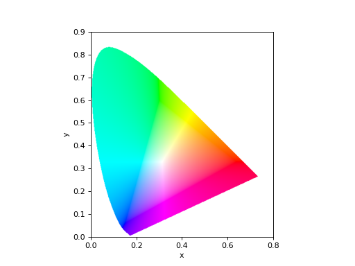
machinevisiontoolbox.base.color.plot_chromaticity_diagram(colorspace='xy', brightness=1, N=500, alpha=1, block=False)

Display chromaticity diagram

Parameters:

• colorspace (string) – colorspace to show: ‘xy’ [default], ‘lab’, ‘ab’

• brightness (float, optional) – for xy this is Y, for ab this is L, defaults to 1

• N (integer, optional) – number of points to sample in the x- and y-directions, defaults to 500

• alpha (float, optional) – alpha value for plot in the range [0,1], defaults to 1

• block (bool) – block until plot is dismissed, defaults to False

Returns:

chromaticity diagram as an image

Return type:

ndarray(N,N,3)

Display, using Matplotlib, a chromaticity diagram as an image using Matplotlib. This is the “horseshoe-shaped” curve bounded by the spectral locus, and internal pixels are an approximation of their true color (at the specified brightness).

Example:

>>> from machinevisiontoolbox import plot_chromaticity_diagram
>>> plot_chromaticity_diagram()  # show filled chromaticity diagram

(Source code, png, hires.png, pdf)

Note

The colors shown within the locus only approximate the true colors, due to the gamut of the display device.

References:

• Robotics, Vision & Control for Python, Section 10.1, P. Corke, Springer 2023.

Seealso:

plot_spectral_locus

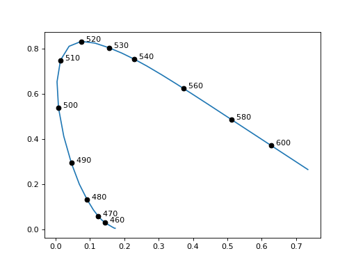
machinevisiontoolbox.base.color.plot_spectral_locus(colorspace='xy', labels=True, ax=None, block=False, lambda_ticks=None)

Plot spectral locus

Parameters:

• colorspace (str, optional) – the color space: ‘xy’ [default] or ‘rg’

• labels (bool, optional) – display wavelength labels, defaults to True

• ax (axes, optional) – Matplotlib axes to draw into, defaults to current

• block (bool, optional) – block until plot is dismissed, defaults to False

• lambda_ticks (array_like, optional) – interval between wavelength labels, defaults to None

Raises:

ValueError – unknown colorspace

Plot, using Matplotlib, the boundary of the “horseshoe” in the chromaticity diagram which represents pure spectral colors. Labelled points are added to the boundary at default spacing, but \(\lambda\) values can be specified by the iterable lambda_ticks.

Typically, would be used in conjunction with plot_chromaticity_diagram to plot chromaticity diagram with labelled boundary.

Example:

>>> from machinevisiontoolbox import plot_spectral_locus
>>> plot_spectral_locus()  # add the border

(Source code, png, hires.png, pdf)

Seealso:

plot_chromaticity_diagram

machinevisiontoolbox.base.color.cie_primaries()

CIE primary wavelengths

cie_primaries is a 3-vector with the wavelengths [m] of the CIE-1976 red, green and blue primaries respectively.

Example:

>>> from machinevisiontoolbox import cie_primaries
>>> cie_primaries()*1e9
array([700. , 546.1, 435.8])

machinevisiontoolbox.base.color.colorspace_convert(image, src, dst)

Convert images between colorspaces

Parameters:

• image (ndarray(H,W,3), (N,3)) – input image

• src (str) – input colorspace name

• dst (str) – output colorspace name

Returns:

output image

Return type:

ndarray(N,M,3), (N,3)

Convert images or rowwise color coordinates from one color space to another. The work is done by OpenCV and assumes that the input image is linear, not gamma encoded, and the result is also linear.

Color space names (synonyms listed on the same line) are:

Color space name	Option string(s)
grey scale	'grey', 'gray'
RGB (red/green/blue)	'rgb'
BGR (blue/green/red)	'bgr'
CIE XYZ	'xyz', 'xyz_709'
YCrCb	'ycrcb'
HSV (hue/sat/value)	'hsv'
HLS (hue/lightness/sat)	'hls'
CIE L*a*b*	'lab', ‘l*a*b*'
CIE L*u*v*	'luv', 'l*u*v*'

Example:

>>> from machinevisiontoolbox import colorspace_convert
>>> colorspace_convert([0, 0, 1], 'rgb', 'hls')
array([240. ,   0.5,   1. ])

Seealso:

gamma_decode cv2.cvtColor

machinevisiontoolbox.base.color.gamma_encode(image, gamma='sRGB')

Gamma encoding

Parameters:

• image (ndarray(H,W), ndarray(H,W,N)) – input image

• gamma (float, str) – gamma exponent or “srgb”

Returns:

gamma encoded version of image

Return type:

ndarray(H,W), ndarray(H,W,N)

Maps linear tristimulus values to a gamma encoded values using either:

• \(y = x^\gamma\)

• the sRGB mapping which is an exponential as above, with a linear segment near zero.

Note

• Gamma encoding should be applied to any image prior to display, since the display assumes the image is gamma encoded. If not encoded, the displayed image will appear very contrasty.

• Gamma encoding is typically performed in a camera with \(\gamma=0.45\).

• For images with multiple planes, the gamma encoding is applied to each plane.

• For images of type double, the pixels are assumed to be in the range 0 to 1.

• For images of type int, the pixels are assumed in the range 0 to the maximum value of their class. Pixels are converted first to double, encoded, then converted back to the integer class.

References:

• Robotics, Vision & Control for Python, Section 10.1, P. Corke, Springer 2023.

Seealso:

gamma_decode colorspace_convert

machinevisiontoolbox.base.color.gamma_decode(image, gamma='sRGB')

Gamma decoding

Parameters:

• image (ndarray(H,W), ndarray(H,W,N)) – input image

• gamma (float, str) – gamma exponent or “srgb”

Returns:

gamma decoded version of image

Return type:

ndarray(H,W), ndarray(H,W,N)

Maps linear tristimulus values to a gamma encoded values using either:

• \(y = x^\gamma\)

• the sRGB mapping which is an exponential as above, with a linear segment near zero.

Note

• Gamma decoding should be applied to any color image prior to colometric operations.

• Gamma decoding is typically performed in the display with \(\gamma=2.2\).

• For images with multiple planes, the gamma correction is applied to each plane.

• For images of type double, the pixels are assumed to be in the range 0 to 1.

• For images of type int, the pixels are assumed in the range 0 to the maximum value of their class. Pixels are converted first to double, encoded, then converted back to the integer class.

References:

• Robotics, Vision & Control for Python, Section 10.1, P. Corke, Springer 2023.

Seealso:

gamma_encode

machinevisiontoolbox.base.color.shadow_invariant(image, θ=None, geometricmean=True, exp=False, sharpen=None, primaries=None)

Shadow invariant image

Parameters:

• image (ndarray(H,W,3) float) – linear color image

• geometricmean (bool, optional) – normalized with geometric mean of color channels, defaults to True

• exp (bool, optional) – exponentiate the logarithmic image, defaults to False

• sharpen (ndarray(3,3), optional) – a sharpening transform, defaults to None

• primaries (array_like(3), optional) – camera peak filter responses (nm), defaults to None

Returns:

greyscale shadow invariant image

Return type:

ndarray(H,W)

Computes the greyscale invariant image computed from the passed color image with a projection line of slope θ.

If θ is not provided then the slope is computed from the camera spectral characteristics primaries a vector of the peak response of the camera’s filters in the order red, green, blue. If these aren’t provided they default to 610, 538, and 460nm.

Example:

>>> im = iread('parks.png', gamma='sRGB', dtype='double')
>>> gs = shadow_invariant(im, 0.7)
>>> idisp(gs)

Note

• The input image is assumed to be linear, that is, it has been gamma decoded.

References:

• “Dealing with shadows: Capturing intrinsic scene appear for image-based outdoor localisation,” P. Corke, R. Paul, W. Churchill, and P. Newman Proc. Int. Conf. Intelligent Robots and Systems (IROS), pp. 2085–2 2013.

• Robotics, Vision & Control for Python, Section 10.1, P. Corke, Springer 2023.

machinevisiontoolbox.base.color.esttheta(im, sharpen=None)

Estimate theta for shadow invariance

Parameters:

• im (ndarray(H,W,3)) – input image

• sharpen (ndarray(3,3), optional) – a sharpening transform, defaults to None

Returns:

the value of θ

Return type:

float

This is an interactive procedure where the image is displayed and the user selects a region of homogeneous material (eg. grass or road) that includes areas that are directly lit by the sun and in shadow.

Note

The user selects boundary points by clicking the mouse. After the last point, hit the Enter key and the region will be closed.