Visualization

Rendering the graph itself, with matplotlib or via GraphViz. See Exporting a graph for exporting the graph as data or an image file (dot, Mermaid, GraphML, ELK, PNG, …) and Transformations to matrix representations for its matrices.

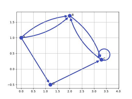
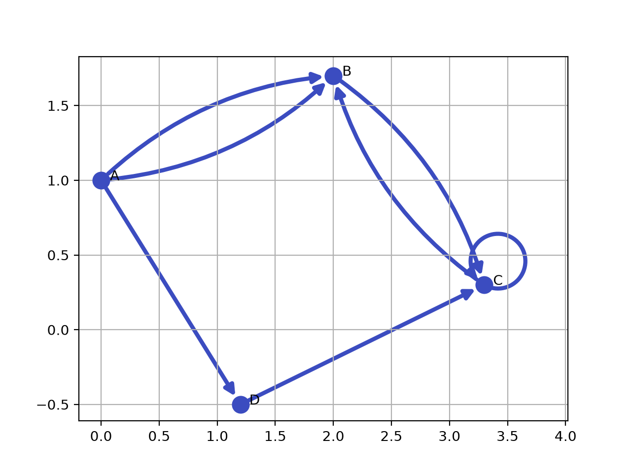
plot() draws each edge once. A directed graph has an arrowhead at the end of each edge, edges that join the same pair of vertices are drawn as arcs that bow apart so that parallel and antiparallel edges can all be seen, and a loop is drawn as a circle at its vertex. The same is true of a 3D plot, which follows a rotation of the view.

The appearance is set by dicts of Matplotlib options:

option	applies to	default
`vertex_opt`	the vertex marker (`plot`)	`marker="o", markersize=12`
`edge_opt`	the edge line (`FancyArrowPatch`): `color`, `linewidth`, `linestyle`, `alpha`	`linewidth=3`
`arrow_opt`	the arrowhead and the path: `arrowstyle`, `mutation_scale`, `connectionstyle`	`arrowstyle="-\|>",` `mutation_scale=15` for a directed graph, `"-"` for an undirected one
`text_opt`	the vertex labels (`text`)	Matplotlib’s

labels=False removes the labels, and color_components=False draws the graph in one color rather than a color for each component.

Note

The options were named vopt, eopt, text, colorcomponents and force2d in 0.6.5. Those names still work but give a DeprecationWarning.

`plot`	Plot graph as a vertex/edge diagram using Matplotlib
`showgraph`	Display graph as a vertex/edge diagram in a browser tab
`highlight_path`	Highlight a path through the graph
`highlight_edge`	Highlight an edge in a plot of the graph
`highlight_vertex`	Highlight a vertex in the graph

Details

Graph.plot(colorcomponents=None, force2d=None, vopt=None, eopt=None, text=None, block=False, grid=True, ax=None, *, vertex_opt=None, edge_opt=None, arrow_opt=None, text_opt=None, labels=None, color_components=None, force_2d=None)[source]

Plot graph as a vertex/edge diagram using Matplotlib

Parameters:

vertex_opt (dict, optional) – vertex format, a dict of Matplotlib plot options, defaults to a 12 point circle marker
edge_opt (dict, optional) – edge format, a dict of Matplotlib patch options such as color, linewidth and linestyle, defaults to a line width of 3
arrow_opt (dict, optional) – arrowhead and path format, a dict of Matplotlib FancyArrowPatch options such as arrowstyle, mutation_scale and connectionstyle, defaults to dict(arrowstyle="-|>", mutation_scale=15) for a directed graph and dict(arrowstyle="-"), no head, for an undirected graph
labels (bool, optional) – label each vertex with its name, defaults to True
text_opt (dict, optional) – format of the labels, a dict of Matplotlib text options
color_components (bool, optional) – color vertices and edges by component, defaults to True
force_2d (bool, optional) – plot only the first two coordinates of each vertex even if they have more, defaults to False
grid (bool, optional) – show a grid, defaults to True
ax (Axes or Axes3D, optional) – axes to draw in, defaults to the current axes or a new figure
block (bool or None, optional) – block until figure is dismissed, defaults to False. If None the figure is not shown at all, which is useful when adding to the plot or saving it.

Raises:

ValueError – the graph is empty, or a vertex has no coordinate or fewer than two coordinate values
TypeError – an option is given by both its old and new name

Return type:

None

The graph is plotted using Matplotlib according to the dimensionality of the vertex coordinates (set by the dim parameter to graph constructor). If the dimensionality is

2, then a 2D plot is generated.
3, then a 3D plot is generated.
4 or more, then a 3D plot is generated using the first three coordinates.

If a vertex has no coordinate or fewer than two values, a ValueError is raised.

Every edge is drawn once. In a directed graph it ends in an arrowhead at its end vertex. Edges that join the same pair of vertices, whichever way they point, are drawn as arcs that bow to either side so that parallel and antiparallel edges can all be seen, and a loop is drawn as a circle at its vertex.

If color_components is True then all edges and vertices within a component are assigned a unique color.

Note

Only embedded graphs can be plotted: every vertex must have a coordinate of at least two values. A coordinate of more than two values is drawn in 3D, using the first three.

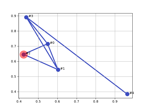
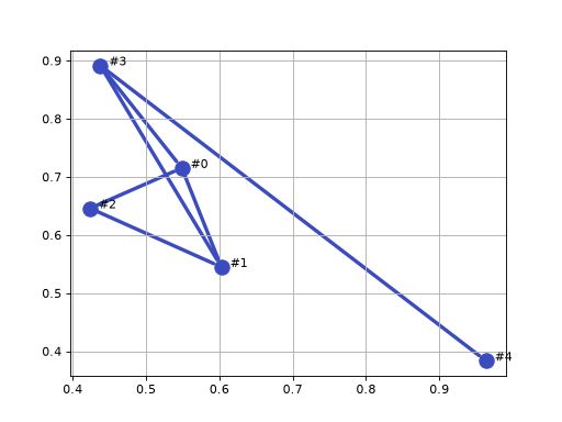
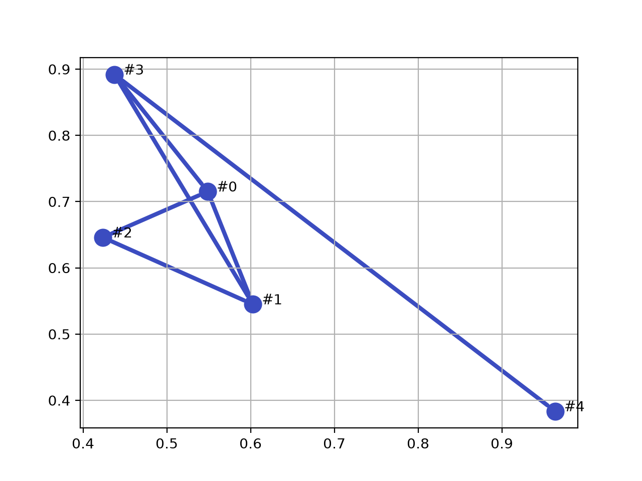
Changed in version 1.0: A directed graph is drawn with arrowheads. In 0.6.5 it was indistinguishable from an undirected one, parallel edges were drawn on top of each other and loops were not visible. The options are named vertex_opt, edge_opt, arrow_opt and text_opt. vopt, eopt, text, colorcomponents and force2d are deprecated: they still work and give a DeprecationWarning. text=False is labels=False and a text dict is text_opt.

>>> from pgraph import UGraph
>>> import numpy as np
>>> np.random.seed(0)
>>> g = UGraph()
>>> for i in range(5):
...     g.add_vertex(np.random.rand(2));
Vertex[#0, coord=(0.5488, 0.7152)]
Vertex[#1, coord=(0.6028, 0.5449)]
Vertex[#2, coord=(0.4237, 0.6459)]
Vertex[#3, coord=(0.4376, 0.8918)]
Vertex[#4, coord=(0.9637, 0.3834)]
>>> for i, j in [(0, 1), (0, 2), (0, 3), (1, 2), (1, 3), (3, 4)]:
...     g.add_edge(g[i], g[j]);
Edge{[#0] -- [#1], cost=0.1786}
Edge{[#0] -- [#2], cost=0.1431}
Edge{[#0] -- [#3], cost=0.2087}
Edge{[#1] -- [#2], cost=0.2056}
Edge{[#1] -- [#3], cost=0.3842}
Edge{[#3] -- [#4], cost=0.7315}
>>> g.plot(block=None)

(Source code, png, hires.png, pdf)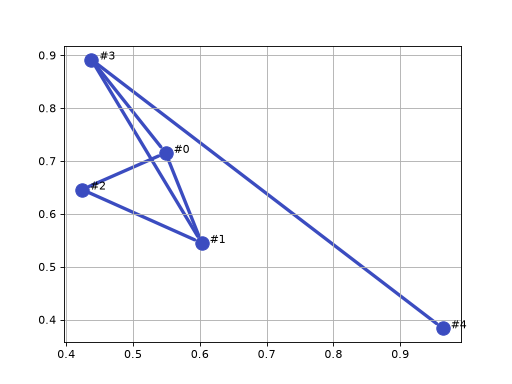

A directed graph, with a pair of antiparallel edges, a pair of parallel edges and a loop

(Source code, png, hires.png, pdf)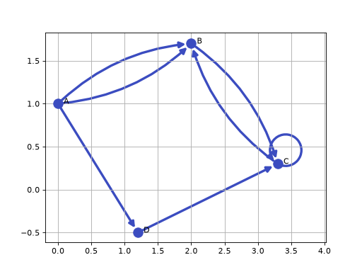

Seealso:: highlight_path() highlight_edge()

Graph.showgraph(display=True, **options)[source]

Display graph as a vertex/edge diagram in a browser tab

Parameters:

display (bool) – open the rendered PDF in a browser tab, defaults to True
options (Any) – engine, direction, color_components and costs, passed to export()

Raises:

RuntimeError – GraphViz is not installed, or fails

Returns:

path of the rendered PDF if display is False, else None

Return type:

str or None

g.showgraph() renders the graph to PDF with GraphViz and displays it in a browser tab. With display=False the PDF is rendered but not opened and its path is returned, which is useful for tests and notebooks.

Note

Vertices do not have to have coordinates for this to work, but if they do the coordinates are used to position the vertices in the output. If no coordinates are given, GraphViz will choose a layout.

Seealso:: export() dotfile()

Graph.highlight_path(path, block=False, **kwargs)[source]

Highlight a path through the graph

Parameters:

path (list of Vertex subclass) – sequence of vertices forming a path
block (bool or None, optional) – block until figure is dismissed, defaults to False. If None the figure is not shown.
kwargs (Any) – arguments passed to highlight_edge() and highlight_vertex()

Return type:

None

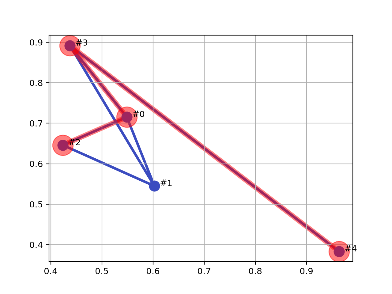
The vertices and edges along the path are overwritten with a different size/width and color.

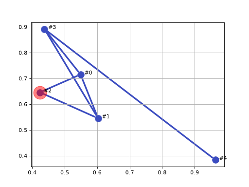
>>> from pgraph import UGraph
>>> import numpy as np
>>> np.random.seed(0)
>>> g = UGraph()
>>> for i in range(5):
...     g.add_vertex(np.random.rand(2));
Vertex[#0, coord=(0.5488, 0.7152)]
Vertex[#1, coord=(0.6028, 0.5449)]
Vertex[#2, coord=(0.4237, 0.6459)]
Vertex[#3, coord=(0.4376, 0.8918)]
Vertex[#4, coord=(0.9637, 0.3834)]
>>> for i, j in [(0, 1), (0, 2), (0, 3), (1, 2), (1, 3), (3, 4)]:
...     g.add_edge(g[i], g[j]);
Edge{[#0] -- [#1], cost=0.1786}
Edge{[#0] -- [#2], cost=0.1431}
Edge{[#0] -- [#3], cost=0.2087}
Edge{[#1] -- [#2], cost=0.2056}
Edge{[#1] -- [#3], cost=0.3842}
Edge{[#3] -- [#4], cost=0.7315}
>>> g.plot(block=None)
>>> path, length, _ = g.path_Astar(g[2], g[4])
>>> g.highlight_path(path, block=None)

(Source code, png, hires.png, pdf)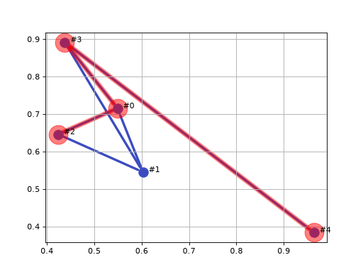

Seealso:: highlight_vertex() highlight_edge()

Graph.highlight_edge(edge, scale=2, color='r', alpha=0.5)[source]

Highlight an edge in a plot of the graph

Parameters:

edge (Edge subclass) – The edge to highlight
scale (float, optional) – Overwrite with a line that is thicker than the original, defaults to 1.5
color (str, optional) – Overwrite with a line in this color, defaults to ‘r’
alpha (float, optional) – Transparency of the highlight, defaults to 0.5

Raises:

ValueError – edge does not connect two vertices, for example because it has been removed from the graph

Return type:

None

>>> from pgraph import UGraph
>>> import numpy as np
>>> np.random.seed(0)
>>> 
>>> g = UGraph()
>>> for i in range(5):
...     g.add_vertex(np.random.rand(2));
Vertex[#0, coord=(0.5488, 0.7152)]
Vertex[#1, coord=(0.6028, 0.5449)]
Vertex[#2, coord=(0.4237, 0.6459)]
Vertex[#3, coord=(0.4376, 0.8918)]
Vertex[#4, coord=(0.9637, 0.3834)]
>>> edges = []
>>> for i, j in [(0, 1), (0, 2), (0, 3), (1, 2), (1, 3), (3, 4)]:
...     edges.append(g.add_edge(g[i], g[j]));
>>> g.plot(block=None)
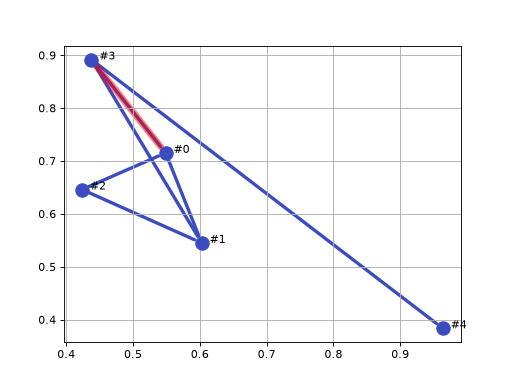
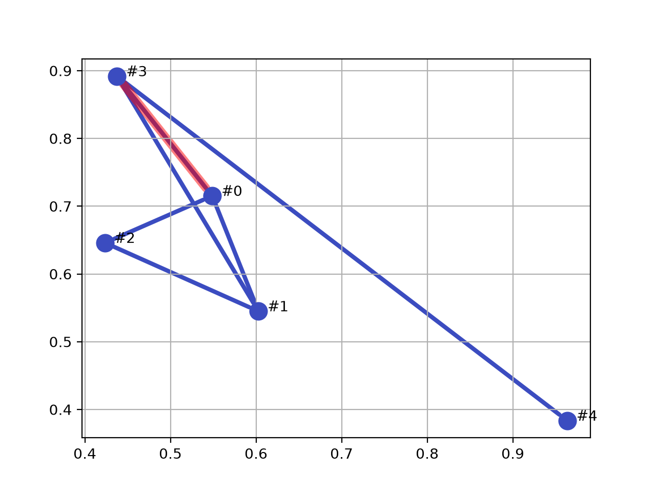
>>> g.highlight_edge(edges[2])

(Source code, png, hires.png, pdf)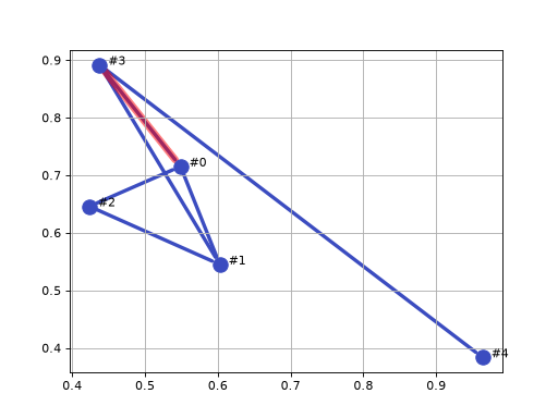

Seealso:: plot() highlight_vertex() highlight_path()

Graph.highlight_vertex(vertex, scale=2, color='r', alpha=0.5)[source]

Highlight a vertex in the graph

Parameters:

vertex (Vertex subclass, or iterable of Vertex subclass or str) – The vertex (or vertices, or vertex names) to highlight
scale (float, optional) – Overwrite with a marker that is larger than the original, defaults to 1.5
color (str, optional) – Overwrite with a line in this color, defaults to ‘r’
alpha (float, optional) – Transparency of the highlight, defaults to 0.5

Return type:

None

>>> from pgraph import UGraph
>>> import numpy as np
>>> np.random.seed(0)
>>> g = UGraph()
>>> for i in range(5):
...     g.add_vertex(np.random.rand(2));
Vertex[#0, coord=(0.5488, 0.7152)]
Vertex[#1, coord=(0.6028, 0.5449)]
Vertex[#2, coord=(0.4237, 0.6459)]
Vertex[#3, coord=(0.4376, 0.8918)]
Vertex[#4, coord=(0.9637, 0.3834)]
>>> for i, j in [(0, 1), (0, 2), (0, 3), (1, 2), (1, 3), (3, 4)]:
...     g.add_edge(g[i], g[j]);
Edge{[#0] -- [#1], cost=0.1786}
Edge{[#0] -- [#2], cost=0.1431}
Edge{[#0] -- [#3], cost=0.2087}
Edge{[#1] -- [#2], cost=0.2056}
Edge{[#1] -- [#3], cost=0.3842}
Edge{[#3] -- [#4], cost=0.7315}
>>> g.plot(block=None)
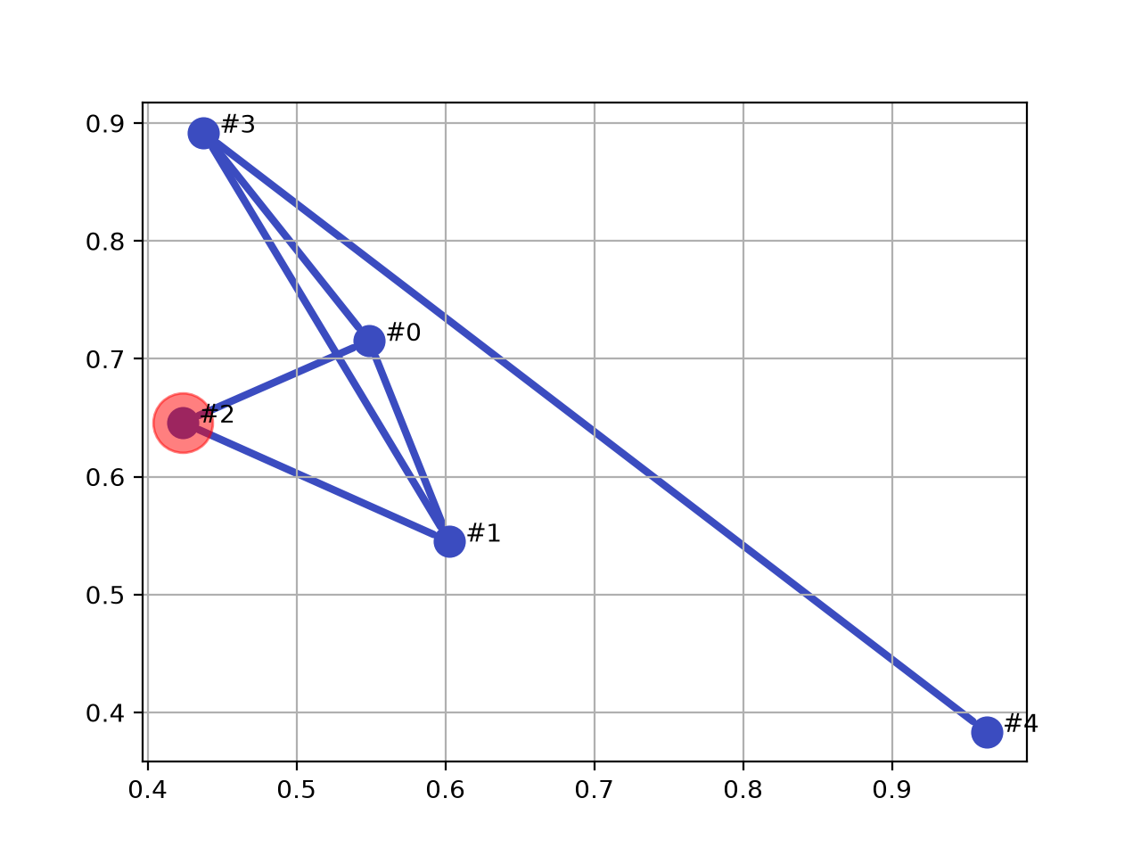
>>> g.highlight_vertex(g[2])

(Source code, png, hires.png, pdf)