
Supporting classes#
Image feature classes#
Whole image features#
Create histogram instance |
Fiducial features#
Properties of a visual fiducial marker |
Blob features#
Line features#
Hough line features |
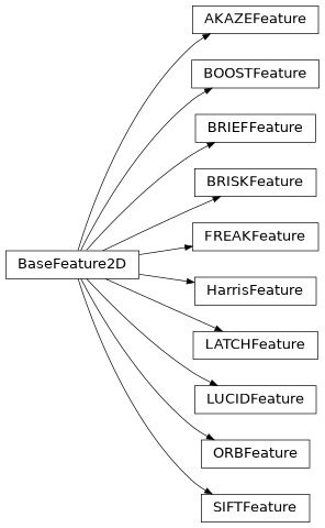
Point features#
A 2D point feature class |
|
Create feature match object |
|
Create set of SIFT point features |
|
Create set of ORB point features |
|
Create set of BRISK point features |
|
Create set of AKAZE point features |
|
Create set of FREAK point features |
|
Create set of BOOST point features |
|
Create set of BRIEF point features |
|
Create set of DAISY point features |
|
Create set of LATCH point features |
|
Create set of LUCID point features |
|
Create set of Harris corner features |
Convolution kernel class#
|
Convolution kernel object |
Bag of words#
Simple bag of words image mathing class
Bag of words class |
Bundle adjustment#
Simple bundle adjustment class
Create a bundle adjustment problem |
|
Create new camera viewpoint |
|
Create new landmark point |
|
Create new landmark observation |