ERobot models

Code author: Jesse Haviland

ERobot

The various models ERobot models all subclass this class.

@author: Jesse Haviland

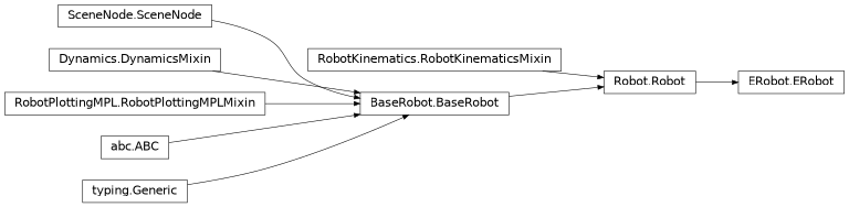
class roboticstoolbox.robot.ERobot.ERobot(*args, **kwargs)[source]

Bases: Robot

classmethod URDF(file_path, gripper=None)

Construct a Robot object from URDF file

Parameters:

file_path (str) – the path to the URDF
gripper (Union[int, str, None]) – index or name of the gripper link(s)

Returns:

If gripper is specified, links from that link outward are removed
from the rigid-body tree and folded into a Gripper object.

static URDF_read(file_path, tld=None, xacro_tld=None)

Read a URDF file as Links

File should be specified relative to RTBDATA/URDF/xacro

Parameters:

file_path – File path relative to the xacro folder
tld – A custom top-level directory which holds the xacro data, defaults to None
xacro_tld – A custom top-level within the xacro data, defaults to None

Return type:

Tuple[List[Link], str, str, Union[Path, PurePosixPath]]

Returns:

links – a list of links
name – the name of the robot
urdf – a string representing the URDF
file_path – a path to the original file

Notes

If tld is not supplied, filepath pointing to xacro data should be directly under RTBDATA/URDF/xacro OR under ./xacro relative to the model file calling this method. If tld is supplied, then `file_path` needs to be relative to tld

__getitem__(i)

Get link

This also supports iterating over each link in the robot object, from the base to the tool.

Parameters:: i (Union[int, str]) – link number or name
Returns:: i’th link or named link
Return type:: link

Examples

>>> import roboticstoolbox as rtb
>>> robot = rtb.models.DH.Puma560()
>>> print(robot[1]) # print the 2nd link
RevoluteDH:   θ=q,  d=0,  a=0.4318,  ⍺=0.0
>>> print([link.a for link in robot])  # print all the a_j values
[0, 0.4318, 0.0203, 0, 0, 0]

Notes

Robot supports link lookup by name,: eg. robot['link1']

__str__()

Pretty prints the ETS Model of the robot.

Returns:: Pretty print of the robot model
Return type:: str

Notes

Constant links are shown in blue.
End-effector links are prefixed with an @
Angles in degrees
The robot base frame is denoted as BASE and is equal to the
robot’s base attribute.

accel(q, qd, torque, gravity=None)

Compute acceleration due to applied torque

qdd = accel(q, qd, torque) calculates a vector (n) of joint accelerations that result from applying the actuator force/torque (n) to the manipulator in state q (n) and qd (n), and n is the number of robot joints.

\[\ddot{q} = \mathbf{M}^{-1} \left(\tau - \mathbf{C}(q)\dot{q} - \mathbf{g}(q)\right)\]

Trajectory operation

If q, qd, torque are matrices (m,n) then qdd is a matrix (m,n) where each row is the acceleration corresponding to the equivalent rows of q, qd, torque.

Parameters:

q – Joint coordinates
qd – Joint velocity
torque – Joint torques of the robot
gravity – Gravitational acceleration (Optional, if not supplied will use the gravity attribute of self).

Return type:

ndarray(n)

Examples

>>> import roboticstoolbox as rtb
>>> puma = rtb.models.DH.Puma560()
>>> puma.accel(puma.qz, 0.5 * np.ones(6), np.zeros(6))
array([ -7.5544, -12.22  ,  -6.4022,  -5.4303,  -4.9518,  -2.1178])

Notes

Useful for simulation of manipulator dynamics, in
conjunction with a numerical integration function.
Uses the method 1 of Walker and Orin to compute the forward
dynamics.
Featherstone’s method is more efficient for robots with large
numbers of joints.
Joint friction is considered.

References

Efficient dynamic computer simulation of robotic mechanisms,
M. W. Walker and D. E. Orin, ASME Journa of Dynamic Systems, Measurement and Control, vol. 104, no. 3, pp. 205-211, 1982.

accel_x(q, xd, wrench, gravity=None, pinv=False, representation='rpy/xyz')

Operational space acceleration due to applied wrench

xdd = accel_x(q, qd, wrench) is the operational space acceleration due to wrench applied to the end-effector of a robot in joint configuration q and joint velocity qd.

\[\ddot{x} = \mathbf{J}(q) \mathbf{M}(q)^{-1} \left( \mathbf{J}(q)^T w - \mathbf{C}(q)\dot{q} - \mathbf{g}(q) \right)\]

Trajectory operation

If q, qd, torque are matrices (m,n) then qdd is a matrix (m,n) where each row is the acceleration corresponding to the equivalent rows of q, qd, wrench.

Parameters:

q – Joint coordinates
qd – Joint velocity
wrench – Wrench applied to the end-effector
gravity – Gravitational acceleration (Optional, if not supplied will use the gravity attribute of self).
pinv – use pseudo inverse rather than inverse
analytical – the type of analytical Jacobian to use, default is ‘rpy/xyz’
xd –
representation – (Default value = “rpy/xyz”)

Returns:

Operational space accelerations of the end-effector

Return type:

accel

Examples

    ainv = _umath_linalg.inv(a, signature=signature, extobj=extobj)
  File "/opt/hostedtoolcache/Python/3.7.16/x64/lib/python3.7/site-packages/numpy/linalg/linalg.py", line 88, in _raise_linalgerror_singular
    raise LinAlgError("Singular matrix")
numpy.linalg.LinAlgError: Singular matrix

Notes

Useful for simulation of manipulator dynamics, in
conjunction with a numerical integration function.
Uses the method 1 of Walker and Orin to compute the forward
dynamics.
Featherstone’s method is more efficient for robots with large
numbers of joints.
Joint friction is considered.

See also

accel()

addconfiguration(name, q)

Add a named joint configuration

Add a named configuration to the robot instance’s dictionary of named configurations.

Parameters:

name (str) – Name of the joint configuration
q (ndarray) – Joint configuration

Examples

>>> import roboticstoolbox as rtb
>>> robot = rtb.models.DH.Puma560()
>>> robot.addconfiguration_attr("mypos", [0.1, 0.2, 0.3, 0.4, 0.5, 0.6])
>>> robot.configs["mypos"]
array([0.1, 0.2, 0.3, 0.4, 0.5, 0.6])

See also

addconfiguration()

addconfiguration_attr(name, q, unit='rad')

Add a named joint configuration as an attribute

Parameters:

name (str) – Name of the joint configuration
q (Union[ndarray, List[float], Tuple[float], Set[float]]) – Joint configuration

Examples

>>> import roboticstoolbox as rtb
>>> robot = rtb.models.DH.Puma560()
>>> robot.addconfiguration_attr("mypos", [0.1, 0.2, 0.3, 0.4, 0.5, 0.6])
>>> robot.mypos
array([0.1, 0.2, 0.3, 0.4, 0.5, 0.6])
>>> robot.configs["mypos"]
array([0.1, 0.2, 0.3, 0.4, 0.5, 0.6])

Notes

Used in robot model init method to store the qr configuration
Dynamically adding attributes to objects can cause issues with
Python type checking.
Configuration is also added to the robot instance’s dictionary of
named configurations.

See also

addconfiguration()

attach(object)

attach_to(object)

property base: SE3

Get/set robot base transform

robot.base is the robot base transform
robot.base = ... checks and sets the robot base transform

Parameters:: base – the new robot base transform
Returns:: the current robot base transform
Return type:: base

property base_link: LinkType

Get the robot base link

robot.base_link is the robot base link

Returns:: the first link in the robot tree
Return type:: base_link

cinertia(q): Deprecated, use inertia_x

closest_point(q, shape, inf_dist=1.0, skip=False)

Find the closest point between robot and shape

closest_point(shape, inf_dist) returns the minimum euclidean distance between this robot and shape, provided it is less than inf_dist. It will also return the points on self and shape in the world frame which connect the line of length distance between the shapes. If the distance is negative then the shapes are collided.

shape: The shape to compare distance to

inf_dist: The minimum distance within which to consider the shape

skip: Skip setting all shape transforms based on q, use this option if using this method in conjuction with Swift to save time

Return type:

Tuple[Optional[int], Optional[ndarray], Optional[ndarray]]

Returns:

d – distance between the robot and shape
p1 – [x, y, z] point on the robot (in the world frame)
p2 – [x, y, z] point on the shape (in the world frame)

collided(q, shape, skip=False)

Check if the robot is in collision with a shape

collided(shape) checks if this robot and shape have collided

shape: The shape to compare distance to

skip: Skip setting all shape transforms based on q, use this option if using this method in conjuction with Swift to save time

Returns:: True if shapes have collided
Return type:: collided

property comment: str

Get/set robot comment

robot.comment is the robot comment
robot.comment = ... checks and sets the robot comment

Parameters:: name – the new robot comment
Returns:: robot comment
Return type:: comment

property configs: Dict[str, ndarray]

configurations_str(border='thin')

property control_mode: str

Get/set robot control mode

robot.control_type is the robot control mode
robot.control_type = ... checks and sets the robot control mode

Parameters:: control_mode – the new robot control mode
Returns:: the current robot control mode
Return type:: control_mode

copy()

coriolis(q, qd)

Coriolis and centripetal term

coriolis(q, qd) calculates the Coriolis/centripetal matrix (n,n) for the robot in configuration q and velocity qd, where n is the number of joints.

The product $\mathbf{C} \dot{q}$ is the vector of joint force/torque due to velocity coupling. The diagonal elements are due to centripetal effects and the off-diagonal elements are due to Coriolis effects. This matrix is also known as the velocity coupling matrix, since it describes the disturbance forces on any joint due to velocity of all other joints.

Trajectory operation

If q and qd are matrices (m,n), each row is interpretted as a joint configuration, and the result (n,n,m) is a 3d-matrix where each plane corresponds to a row of q and qd.

Parameters:

q – Joint coordinates
qd – Joint velocity

Returns:

Velocity matrix

Return type:

coriolis

Examples

>>> import roboticstoolbox as rtb
>>> puma = rtb.models.DH.Puma560()
>>> puma.coriolis(puma.qz, 0.5 * np.ones((6,)))
array([[-0.4017, -0.5513, -0.2025, -0.0007, -0.0013,  0.    ],
       [ 0.2023, -0.1937, -0.3868, -0.    , -0.002 ,  0.    ],
       [ 0.1987,  0.193 , -0.    ,  0.    , -0.0001,  0.    ],
       [ 0.    ,  0.    ,  0.    ,  0.    ,  0.    ,  0.    ],
       [ 0.0007,  0.0007,  0.0001,  0.    ,  0.    ,  0.    ],
       [ 0.    ,  0.    ,  0.    ,  0.    ,  0.    ,  0.    ]])

Notes

Joint viscous friction is also a joint force proportional to
velocity but it is eliminated in the computation of this value.
Computationally slow, involves $n^2/2$ invocations of RNE.

coriolis_x(q, qd, pinv=False, representation='rpy/xyz', J=None, Ji=None, Jd=None, C=None, Mx=None)

Operational space Coriolis and centripetal term

coriolis_x(q, qd) is the Coriolis/centripetal matrix (m,m) in operational space for the robot in configuration q and velocity qd, where n is the number of joints.

\[\mathbf{C}_x = \mathbf{J}(q)^{-T} \left( \mathbf{C}(q) - \mathbf{M}_x(q) \mathbf{J})(q) \right) \mathbf{J}(q)^{-1}\]

The product $\mathbf{C} \dot{x}$ is the operational space wrench due to joint velocity coupling. This matrix is also known as the velocity coupling matrix, since it describes the disturbance forces on any joint due to velocity of all other joints.

The transformation to operational space requires an analytical, rather than geometric, Jacobian. analytical can be one of:

Value

Rotational representation

'rpy/xyz'

RPY angular rates in XYZ order (default)

'rpy/zyx'

RPY angular rates in XYZ order

'eul'

Euler angular rates in ZYZ order

'exp'

exponential coordinate rates

Trajectory operation

If q and qd are matrices (m,n), each row is interpretted as a joint configuration, and the result (n,n,m) is a 3d-matrix where each plane corresponds to a row of q and qd.

Parameters:

q – Joint coordinates
qd – Joint velocity
pinv – use pseudo inverse rather than inverse (Default value = False)
analytical – the type of analytical Jacobian to use, default is ‘rpy/xyz’
representation – (Default value = “rpy/xyz”)
J –
Ji –
Jd –
C –
Mx –

Returns:

Operational space velocity matrix

Return type:

ndarray(6,6) or ndarray(m,6,6)

Examples

    ainv = _umath_linalg.inv(a, signature=signature, extobj=extobj)
  File "/opt/hostedtoolcache/Python/3.7.16/x64/lib/python3.7/site-packages/numpy/linalg/linalg.py", line 88, in _raise_linalgerror_singular
    raise LinAlgError("Singular matrix")
numpy.linalg.LinAlgError: Singular matrix

Notes

Joint viscous friction is also a joint force proportional to
velocity but it is eliminated in the computation of this value.
Computationally slow, involves $n^2/2$ invocations of RNE.
If the robot is not 6 DOF the pinv option is set True.
pinv() is around 5x slower than inv()

Warning

Assumes that the operational space has 6 DOF.

property default_backend

Get default graphical backend

robot.default_backend Get the default graphical backend, used when
no explicit backend is passed to Robot.plot.
robot.default_backend = ... Set the default graphical backend, used when
no explicit backend is passed to Robot.plot. The default set here will be overridden if the particular Robot subclass cannot support it.

Returns:: backend name
Return type:: default_backend

dfs_links(start, func=None)

A link search method

Visit all links from start in depth-first order and will apply func to each visited link

Parameters:

start (TypeVar(LinkType, bound= BaseLink)) – The link to start at
func (Optional[Callable[[TypeVar(LinkType, bound= BaseLink)], Any]]) – An optional function to apply to each link as it is found

Returns:

A list of links

Return type:

links

dotfile(filename, etsbox=False, ets='full', jtype=False, static=True)

Write a link transform graph as a GraphViz dot file

The file can be processed using dot:

% dot -Tpng -o out.png dotfile.dot

The nodes are:

Base is shown as a grey square. This is the world frame origin, but can be changed using the base attribute of the robot.
Link frames are indicated by circles
ETS transforms are indicated by rounded boxes

The edges are:

an arrow if jtype is False or the joint is fixed
an arrow with a round head if jtype is True and the joint is revolute
an arrow with a box head if jtype is True and the joint is prismatic

Edge labels or nodes in blue have a fixed transformation to the preceding link.

Note

If filename is a file object then the file will not: be closed after the GraphViz model is written.

Parameters:

file – Name of file to write to
etsbox (bool) – Put the link ETS in a box, otherwise an edge label
ets (Literal['full', 'brief']) – Display the full ets with “full” or a brief version with “brief”
jtype (bool) – Arrowhead to node indicates revolute or prismatic type
static (bool) – Show static joints in blue and bold

See also

showgraph()

dynamics()

Pretty print the dynamic parameters (Robot superclass)

The dynamic parameters (inertial and friction) are printed in a table, with one row per link.

Examples

dynamics_list()

Print dynamic parameters (Robot superclass)

Display the kinematic and dynamic parameters to the console in reable format

dynchanged(what=None)

Dynamic parameters have changed

Called from a property setter to inform the robot that the cache of dynamic parameters is invalid.

See also

roboticstoolbox.Link._listen_dyn()

property ee_links: List[LinkType]

ets(start=None, end=None)

Robot to ETS

robot.ets() is an ETS representing the kinematics from base to end-effector.

robot.ets(end=link) is an ETS representing the kinematics from base to the link link specified as a Link reference or a name.

robot.ets(start=l1, end=l2) is an ETS representing the kinematics from link l1 to link l2.

:param : :type : param start: start of path, defaults to base_link :param : :type : param end: end of path, defaults to end-effector

Raises:

ValueError – a link does not belong to this ERobot
TypeError – a bad link argument

Returns:

elementary transform sequence

Return type:

ets

Examples

>>> import roboticstoolbox as rtb
>>> panda = rtb.models.ETS.Panda()
>>> panda.ets()
[ET.tz(eta=0.333), ET.Rz(jindex=0), ET.Rx(eta=-1.5707963267948966), ET.Rz(jindex=1), ET.Rx(eta=1.5707963267948966), ET.tz(eta=0.316), ET.Rz(jindex=2), ET.tx(eta=0.0825), ET.Rx(eta=1.5707963267948966), ET.Rz(jindex=3), ET.tx(eta=-0.0825), ET.Rx(eta=-1.5707963267948966), ET.tz(eta=0.384), ET.Rz(jindex=4), ET.Rx(eta=1.5707963267948966), ET.Rz(jindex=5), ET.tx(eta=0.088), ET.Rx(eta=1.5707963267948966), ET.tz(eta=0.107), ET.Rz(jindex=6), ET.tz(eta=0.10300000000000001), ET.Rz(eta=-0.7853981633974483)]

fdyn(T, q0, Q=None, Q_args={}, qd0=None, solver='RK45', solver_args={}, dt=None, progress=False)

Integrate forward dynamics

tg = R.fdyn(T, q) integrates the dynamics of the robot with zero input torques over the time interval 0 to T and returns the trajectory as a namedtuple with elements:

t the time vector (M,)
q the joint coordinates (M,n)
qd the joint velocities (M,n)

tg = R.fdyn(T, q, torqfun) as above but the torque applied to the joints is given by the provided function:

tau = function(robot, t, q, qd, **args)

where the inputs are:

the robot object

current time

current joint coordinates (n,)

current joint velocity (n,)

args, optional keyword arguments can be specified, these are

passed in from the targs kewyword argument.

The function must return a Numpy array (n,) of joint forces/torques.

Parameters:

T (float) – integration time
q0 (Union[ndarray, List[float], Tuple[float], Set[float]]) – initial joint coordinates
qd0 (Union[ndarray, List[float], Tuple[float], Set[float], None]) – initial joint velocities, assumed zero if not given
Q (Optional[Callable[[Any, float, ndarray, ndarray], ndarray]]) – a function that computes generalized joint force as a function of time and/or state
Q_args (Dict) – positional arguments passed to torque
solver (str) – str
solver_args (Dict) – dict
dt (Optional[float]) – float
progress (bool) – show progress bar, default False

Returns:

robot trajectory

Return type:

trajectory

Examples

To apply zero joint torque to the robot without Coulomb friction:

>>> def myfunc(robot, t, q, qd):
>>>     return np.zeros((robot.n,))

>>> tg = robot.nofriction().fdyn(5, q0, myfunc)

>>> plt.figure()
>>> plt.plot(tg.t, tg.q)
>>> plt.show()

We could also use a lambda function:

>>> tg = robot.nofriction().fdyn(
>>>     5, q0, lambda r, t, q, qd: np.zeros((r.n,)))

The robot is controlled by a PD controller. We first define a function to compute the control which has additional parameters for the setpoint and control gains (qstar, P, D):

>>> def myfunc(robot, t, q, qd, qstar, P, D):
>>>     return (qstar - q) * P + qd * D  # P, D are (6,)

>>> tg = robot.fdyn(10, q0, myfunc, torque_args=(qstar, P, D)) )

Many integrators have variable step length which is problematic if we want to animate the result. If dt is specified then the solver results are interpolated in time steps of dt.

Notes

This function performs poorly with non-linear joint friction,
such as Coulomb friction. The R.nofriction() method can be used to set this friction to zero.
If the function is not specified then zero force/torque is
applied to the manipulator joints.
Interpolation is performed using `ScipY integrate.ode
<https://docs.scipy.org/doc/scipy/reference/generated/scipy.integrate.ode.html>`
The SciPy RK45 integrator is used by default
Interpolation is performed using `SciPy interp1
<https://docs.scipy.org/doc/scipy/reference/generated/scipy.interpolate.interp1d.html>`

See also

DHRobot.accel(), DHRobot.nofriction(), DHRobot.rne()

fellipse(q, opt='trans', unit='rad', centre=[0, 0, 0])

Create a force ellipsoid object for plotting with PyPlot

robot.fellipse(q) creates a force ellipsoid for the robot at pose q. The ellipsoid is centered at the origin.

q: The joint configuration of the robot.

opt: ‘trans’ or ‘rot’ will plot either the translational or rotational force ellipsoid

unit: ‘rad’ or ‘deg’ will plot the ellipsoid in radians or degrees

centre: The centre of the ellipsoid, either ‘ee’ for the end-effector or a 3-vector [x, y, z] in the world frame

Returns:: An EllipsePlot object
Return type:: env

Notes

By default the ellipsoid related to translational motion is
drawn. Use opt='rot' to draw the rotational velocity ellipsoid.
By default the ellipsoid is drawn at the origin. The option
centre allows its origin to set to set to the specified 3-vector, or the string “ee” ensures it is drawn at the end-effector position.

fkine(q, end=None, start=None, tool=None, include_base=True)

Forward kinematics

T = robot.fkine(q) evaluates forward kinematics for the robot at joint configuration q.

Trajectory operation: If q has multiple rows (mxn), it is considered a trajectory and the result is an SE3 instance with m values.

q: Joint coordinates

end: end-effector or gripper to compute forward kinematics to

start: the link to compute forward kinematics from

tool: tool transform, optional

Return type:: SE3
Returns:: The transformation matrix representing the pose of the end-effector

Examples

The following example makes a panda robot object, and solves for the forward kinematics at the listed configuration.

>>> import roboticstoolbox as rtb
>>> panda = rtb.models.Panda()
>>> panda.fkine([0, -0.3, 0, -2.2, 0, 2, 0.7854])
SE3(array([[ 0.995 , -0.    ,  0.0998,  0.484 ],
           [-0.    , -1.    ,  0.    ,  0.    ],
           [ 0.0998, -0.    , -0.995 ,  0.4126],
           [ 0.    ,  0.    ,  0.    ,  1.    ]]))

Notes

For a robot with a single end-effector there is no need to
specify end
For a robot with multiple end-effectors, the end must
be specified.
The robot’s base tool transform, if set, is incorporated
into the result.
A tool transform, if provided, is incorporated into the result.
Works from the end-effector link to the base

References

J. Haviland, and P. Corke. “Manipulator Differential Kinematics Part I: Kinematics, Velocity, and Applications.” arXiv preprint arXiv:2207.01796 (2022).
J. Haviland, and P. Corke. “Manipulator Differential Kinematics Part II: Acceleration and Advanced Applications.” arXiv preprint arXiv:2207.01794 (2022).

fkine_all(q)

Compute the pose of every link frame

T = robot.fkine_all(q) is an SE3 instance with robot.nlinks + 1 values:

T[0] is the base transform
T[i] is the pose of link whose number is i

Parameters:: q (Union[ndarray, List[float], Tuple[float], Set[float]]) – The joint configuration
Returns:: Pose of all links
Return type:: fkine_all

References

J. Haviland, and P. Corke. “Manipulator Differential Kinematics Part I: Kinematics, Velocity, and Applications.” arXiv preprint arXiv:2207.01796 (2022).

friction(qd)

Manipulator joint friction (Robot superclass)

robot.friction(qd) is a vector of joint friction forces/torques for the robot moving with joint velocities qd.

The friction model includes:

Viscous friction which is a linear function of velocity.
Coulomb friction which is proportional to sign(qd).

\[\begin{split}\tau_j = G^2 B \dot{q}_j + |G_j| \left\{ \begin{array}{ll} \tau_{C,j}^+ & \mbox{if $\dot{q}_j > 0$} \\ \tau_{C,j}^- & \mbox{if $\dot{q}_j < 0$} \end{array} \right.\end{split}\]

Parameters:: qd (ndarray) – The joint velocities of the robot
Returns:: The joint friction forces/torques for the robot
Return type:: friction

Notes

The friction value should be added to the motor output torque to
determine the nett torque. It has a negative value when qd > 0.
The returned friction value is referred to the output of the
gearbox.
The friction parameters in the Link object are referred to the
motor.
Motor viscous friction is scaled up by $G^2$.
Motor Coulomb friction is scaled up by math:G.
The appropriate Coulomb friction value to use in the
non-symmetric case depends on the sign of the joint velocity, not the motor velocity.
Coulomb friction is zero for zero joint velocity, stiction is
not modeled.
The absolute value of the gear ratio is used. Negative gear
ratios are tricky: the Puma560 robot has negative gear ratio for joints 1 and 3.
The absolute value of the gear ratio is used. Negative gear
ratios are tricky: the Puma560 has negative gear ratio for joints 1 and 3.

See also

Robot.nofriction(), Link.friction()

get_path(end=None, start=None)

Find a path from start to end

Parameters:

end (Union[Gripper, TypeVar(LinkType, bound= BaseLink), str, None]) – end-effector or gripper to compute forward kinematics to
start (Union[Gripper, TypeVar(LinkType, bound= BaseLink), str, None]) – name or reference to a base link, defaults to None

Raises:

ValueError – link not known or ambiguous

Return type:

Tuple[List[TypeVar(LinkType, bound= BaseLink)], int, SE3]

Returns:

path – the path from start to end
n – the number of joints in the path
T – the tool transform present after end

property gravity: ndarray

Get/set default gravitational acceleration (Robot superclass)

robot.name is the default gravitational acceleration
robot.name = ... checks and sets default gravitational
acceleration

Parameters:: gravity – the new gravitational acceleration for this robot
Returns:: gravitational acceleration
Return type:: gravity

Notes

If the z-axis is upward, out of the Earth, this should be a positive number.

gravload(q=None, gravity=None)

Compute gravity load

robot.gravload(q) calculates the joint gravity loading (n) for the robot in the joint configuration q and using the default gravitational acceleration specified in the DHRobot object.

robot.gravload(q, gravity=g) as above except the gravitational acceleration is explicitly specified as g.

Trajectory operation

If q is a matrix (nxm) each column is interpreted as a joint configuration vector, and the result is a matrix (nxm) each column being the corresponding joint torques.

Parameters:

q (Union[ndarray, List[float], Tuple[float], Set[float], None]) – Joint coordinates
gravity (ndarray(3)) – Gravitational acceleration (Optional, if not supplied will use the stored gravity values).

Returns:

The generalised joint force/torques due to gravity

Return type:

gravload

Examples

>>> import roboticstoolbox as rtb
>>> puma = rtb.models.DH.Puma560()
>>> puma.gravload(puma.qz)
array([ 0.    , 37.4837,  0.2489,  0.    ,  0.    ,  0.    ])

gravload_x(q=None, gravity=None, pinv=False, representation='rpy/xyz', Ji=None)

Operational space gravity load

robot.gravload_x(q) calculates the gravity wrench for the robot in the joint configuration q and using the default gravitational acceleration specified in the robot object.

robot.gravload_x(q, gravity=g) as above except the gravitational acceleration is explicitly specified as g.

\[\mathbf{G}_x = \mathbf{J}(q)^{-T} \mathbf{G}(q)\]

The transformation to operational space requires an analytical, rather than geometric, Jacobian. analytical can be one of:

Value

Rotational representation

'rpy/xyz'

RPY angular rates in XYZ order (default)

'rpy/zyx'

RPY angular rates in XYZ order

'eul'

Euler angular rates in ZYZ order

'exp'

exponential coordinate rates

Trajectory operation

If q is a matrix (nxm) each column is interpreted as a joint configuration vector, and the result is a matrix (nxm) each column being the corresponding joint torques.

Parameters:

q – Joint coordinates
gravity – Gravitational acceleration (Optional, if not supplied will use the gravity attribute of self).
pinv – use pseudo inverse rather than inverse (Default value = False)
analytical – the type of analytical Jacobian to use, default is ‘rpy/xyz’
representation – (Default value = “rpy/xyz”)
Ji –

Returns:

The operational space gravity wrench

Return type:

gravload

Examples

    ainv = _umath_linalg.inv(a, signature=signature, extobj=extobj)
  File "/opt/hostedtoolcache/Python/3.7.16/x64/lib/python3.7/site-packages/numpy/linalg/linalg.py", line 88, in _raise_linalgerror_singular
    raise LinAlgError("Singular matrix")
numpy.linalg.LinAlgError: Singular matrix

Notes

If the robot is not 6 DOF the pinv option is set True.
pinv() is around 5x slower than inv()

Warning

Assumes that the operational space has 6 DOF.

See also

gravload()

property grippers: List[Gripper]

Grippers attached to the robot

Returns:: A list of grippers
Return type:: grippers

property hascollision

Robot has collision model

Returns:

hascollision – Robot has collision model
At least one link has associated collision model.

Examples

>>> import roboticstoolbox as rtb
>>> robot = rtb.models.DH.Puma560()
>>> robot.hascollision
False

See also

hasgeometry()

property hasdynamics

Robot has dynamic parameters

Returns:

hasdynamics – Robot has dynamic parameters
At least one link has associated dynamic parameters.

Examples

property hasgeometry

Robot has geometry model

At least one link has associated mesh to describe its shape.

Returns:: Robot has geometry model
Return type:: hasgeometry

Examples

>>> import roboticstoolbox as rtb
>>> robot = rtb.models.DH.Puma560()
>>> robot.hasgeometry
True

See also

hascollision()

hessian0(q=None, end=None, start=None, J0=None, tool=None)

Manipulator Hessian

The manipulator Hessian tensor maps joint acceleration to end-effector spatial acceleration, expressed in the start frame. This function calulcates this based on the ETS of the robot. One of J0 or q is required. Supply J0 if already calculated to save computation time

Parameters:

q – The joint angles/configuration of the robot (Optional, if not supplied will use the stored q values).
end (Union[str, Link, Gripper, None]) – the final link/Gripper which the Hessian represents
start (Union[str, Link, Gripper, None]) – the first link which the Hessian represents
J0 – The manipulator Jacobian in the start frame
tool (Union[ndarray, SE3, None]) – a static tool transformation matrix to apply to the end of end, defaults to None

Returns:

The manipulator Hessian in the start frame

Return type:

h0

Synopsis

This method computes the manipulator Hessian in the start frame. If we take the time derivative of the differential kinematic relationship .. math:

\nu    &= \mat{J}(\vec{q}) \dvec{q} \\
\alpha &= \dmat{J} \dvec{q} + \mat{J} \ddvec{q}

where .. math:

\dmat{J} = \mat{H} \dvec{q}

and $\mat{H} \in \mathbb{R}^{6\times n \times n}$ is the Hessian tensor.

The elements of the Hessian are .. math:

\mat{H}_{i,j,k} =  \frac{d^2 u_i}{d q_j d q_k}

where $u = \{t_x, t_y, t_z, r_x, r_y, r_z\}$ are the elements of the spatial velocity vector.

Similarly, we can write .. math:

\mat{J}_{i,j} = \frac{d u_i}{d q_j}

Examples

The following example makes a Panda robot object, and solves for the base frame Hessian at the given joint angle configuration

>>> import roboticstoolbox as rtb
>>> panda = rtb.models.Panda()
>>> panda.hessian0([0, -0.3, 0, -2.2, 0, 2, 0.7854])
array([[[-0.484 , -0.    , -0.486 , -0.    , -0.1547,  0.    , -0.    ],
        [ 0.    ,  0.0796,  0.    ,  0.2466,  0.    ,  0.2006,  0.    ],
        [ 0.    ,  0.    ,  0.    ,  0.    ,  0.    ,  0.    ,  0.    ],
        [ 0.    , -1.    , -0.    ,  1.    ,  0.    ,  1.    ,  0.    ],
        [ 0.    , -0.    , -0.2955, -0.    ,  0.9463, -0.    ,  0.0998],
        [ 0.    ,  0.    , -0.    , -0.    ,  0.    , -0.    ,  0.    ]],

       [[-0.    , -0.484 , -0.    ,  0.4986, -0.    ,  0.1086,  0.    ],
        [ 0.0796,  0.    ,  0.    ,  0.    ,  0.    ,  0.    ,  0.    ],
        [ 0.    , -0.0796, -0.    , -0.2466, -0.    , -0.2006, -0.    ],
        [ 0.    ,  0.    ,  0.9553,  0.    , -0.3233,  0.    , -0.995 ],
        [ 0.    ,  0.    , -0.    , -0.    ,  0.    , -0.    ,  0.    ],
        [ 0.    ,  0.    ,  0.2955,  0.    , -0.9463,  0.    , -0.0998]],

       [[-0.486 , -0.    , -0.4643, -0.    , -0.1478,  0.    ,  0.    ],
        [ 0.    ,  0.    ,  0.    ,  0.383 ,  0.    ,  0.2237,  0.    ],
        [ 0.    , -0.    , -0.1436, -0.    , -0.0457, -0.    , -0.    ],
        [ 0.    ,  0.    ,  0.    ,  0.9553,  0.    ,  0.9553,  0.    ],
        [ 0.    ,  0.    ,  0.    , -0.    ,  0.8085, -0.    , -0.1987],
        [ 0.    ,  0.    ,  0.    ,  0.2955,  0.    ,  0.2955,  0.    ]],

       [[-0.    ,  0.4986, -0.    , -0.4986,  0.    , -0.1086, -0.    ],
        [ 0.2466,  0.    ,  0.383 ,  0.    ,  0.    ,  0.    ,  0.    ],
        [ 0.    , -0.2466, -0.    ,  0.2466,  0.    ,  0.2006,  0.    ],
        [ 0.    ,  0.    ,  0.    ,  0.    ,  0.3233,  0.    ,  0.995 ],
        [ 0.    ,  0.    ,  0.    ,  0.    ,  0.    ,  0.    , -0.    ],
        [ 0.    ,  0.    ,  0.    ,  0.    ,  0.9463,  0.    ,  0.0998]],

       [[-0.1547, -0.    , -0.1478,  0.    ,  0.05  , -0.    ,  0.    ],
        [ 0.    ,  0.    ,  0.    ,  0.    ,  0.    , -0.1676, -0.    ],
        [ 0.    , -0.    , -0.0457,  0.    ,  0.1464,  0.    ,  0.    ],
        [ 0.    ,  0.    ,  0.    ,  0.    ,  0.    , -0.3233,  0.    ],
        [ 0.    ,  0.    ,  0.    ,  0.    ,  0.    , -0.    ,  0.9093],
        [ 0.    ,  0.    ,  0.    ,  0.    ,  0.    , -0.9463, -0.    ]],

       [[ 0.    ,  0.1086,  0.    , -0.1086, -0.    , -0.1086, -0.    ],
        [ 0.2006,  0.    ,  0.2237,  0.    , -0.1676,  0.    ,  0.    ],
        [ 0.    , -0.2006, -0.    ,  0.2006,  0.    ,  0.2006,  0.    ],
        [ 0.    ,  0.    ,  0.    ,  0.    ,  0.    ,  0.    ,  0.995 ],
        [ 0.    ,  0.    ,  0.    ,  0.    ,  0.    ,  0.    , -0.    ],
        [ 0.    ,  0.    ,  0.    ,  0.    ,  0.    ,  0.    ,  0.0998]],

       [[-0.    ,  0.    ,  0.    , -0.    ,  0.    , -0.    ,  0.    ],
        [ 0.    ,  0.    ,  0.    ,  0.    , -0.    ,  0.    , -0.    ],
        [ 0.    , -0.    , -0.    ,  0.    ,  0.    ,  0.    ,  0.    ],
        [ 0.    ,  0.    ,  0.    ,  0.    ,  0.    ,  0.    ,  0.    ],
        [ 0.    ,  0.    ,  0.    ,  0.    ,  0.    ,  0.    ,  0.    ],
        [ 0.    ,  0.    ,  0.    ,  0.    ,  0.    ,  0.    ,  0.    ]]])

References

J. Haviland, and P. Corke. “Manipulator Differential Kinematics Part I: Kinematics, Velocity, and Applications.” arXiv preprint arXiv:2207.01796 (2022).
J. Haviland, and P. Corke. “Manipulator Differential Kinematics Part II: Acceleration and Advanced Applications.” arXiv preprint arXiv:2207.01794 (2022).

hessiane(q=None, end=None, start=None, Je=None, tool=None)

Manipulator Hessian

The manipulator Hessian tensor maps joint acceleration to end-effector spatial acceleration, expressed in the end coordinate frame. This function calulcates this based on the ETS of the robot. One of J0 or q is required. Supply J0 if already calculated to save computation time

Parameters:

q – The joint angles/configuration of the robot (Optional, if not supplied will use the stored q values).
end (Union[str, Link, Gripper, None]) – the final link/Gripper which the Hessian represents
start (Union[str, Link, Gripper, None]) – the first link which the Hessian represents
J0 – The manipulator Jacobian in the end frame
tool (Union[ndarray, SE3, None]) – a static tool transformation matrix to apply to the end of end, defaults to None

Returns:

The manipulator Hessian in end frame

Return type:

he

Synopsis

This method computes the manipulator Hessian in the end frame. If we take the time derivative of the differential kinematic relationship .. math:

\nu    &= \mat{J}(\vec{q}) \dvec{q} \\
\alpha &= \dmat{J} \dvec{q} + \mat{J} \ddvec{q}

where .. math:

\dmat{J} = \mat{H} \dvec{q}

and $\mat{H} \in \mathbb{R}^{6\times n \times n}$ is the Hessian tensor.

The elements of the Hessian are .. math:

\mat{H}_{i,j,k} =  \frac{d^2 u_i}{d q_j d q_k}

where $u = \{t_x, t_y, t_z, r_x, r_y, r_z\}$ are the elements of the spatial velocity vector.

Similarly, we can write .. math:

\mat{J}_{i,j} = \frac{d u_i}{d q_j}

Examples

The following example makes a Panda robot object, and solves for the end-effector frame Hessian at the given joint angle configuration

>>> import roboticstoolbox as rtb
>>> panda = rtb.models.Panda()
>>> panda.hessiane([0, -0.3, 0, -2.2, 0, 2, 0.7854])
array([[[-0.4816, -0.    , -0.4835, -0.    , -0.1539, -0.    ,  0.    ],
        [ 0.    , -0.0796,  0.    , -0.2466,  0.    , -0.2006,  0.    ],
        [-0.0483, -0.    , -0.0485, -0.    , -0.0154, -0.    ,  0.    ],
        [ 0.    , -0.995 ,  0.    ,  0.995 , -0.    ,  0.995 , -0.    ],
        [ 0.    ,  0.    ,  0.2955, -0.    , -0.9463, -0.    , -0.0998],
        [ 0.    , -0.0998,  0.    ,  0.0998, -0.    ,  0.0998,  0.    ]],

       [[-0.    , -0.4896, -0.    ,  0.4715, -0.    ,  0.088 ,  0.    ],
        [-0.0796,  0.    ,  0.    , -0.    ,  0.    , -0.    ,  0.    ],
        [-0.    ,  0.0309,  0.    ,  0.2952,  0.    ,  0.2104, -0.    ],
        [ 0.    ,  0.    ,  0.9801,  0.    , -0.4161,  0.    , -1.    ],
        [ 0.    ,  0.    , -0.    , -0.    ,  0.    , -0.    ,  0.    ],
        [ 0.    ,  0.    , -0.1987, -0.    ,  0.9093, -0.    ,  0.    ]],

       [[-0.4835, -0.    , -0.4763, -0.    , -0.1516, -0.    ,  0.    ],
        [ 0.    ,  0.    ,  0.    , -0.383 ,  0.    , -0.2237,  0.    ],
        [-0.0485,  0.    ,  0.0965, -0.    ,  0.0307, -0.    ,  0.    ],
        [ 0.    ,  0.    ,  0.    ,  0.9801, -0.    ,  0.9801,  0.    ],
        [ 0.    ,  0.    ,  0.    , -0.    , -0.8085, -0.    ,  0.1987],
        [ 0.    ,  0.    ,  0.    , -0.1987, -0.    , -0.1987, -0.    ]],

       [[-0.    ,  0.4715, -0.    , -0.4715,  0.    , -0.088 ,  0.    ],
        [-0.2466, -0.    , -0.383 ,  0.    , -0.    ,  0.    , -0.    ],
        [-0.    ,  0.2952, -0.    , -0.2952, -0.    , -0.2104,  0.    ],
        [ 0.    ,  0.    ,  0.    ,  0.    ,  0.4161,  0.    ,  1.    ],
        [ 0.    ,  0.    ,  0.    ,  0.    , -0.    ,  0.    , -0.    ],
        [ 0.    ,  0.    ,  0.    ,  0.    , -0.9093,  0.    ,  0.    ]],

       [[-0.1539, -0.    , -0.1516,  0.    ,  0.0644,  0.    , -0.    ],
        [ 0.    ,  0.    ,  0.    , -0.    , -0.    ,  0.1676, -0.    ],
        [-0.0154,  0.    ,  0.0307, -0.    , -0.1407, -0.    ,  0.    ],
        [ 0.    ,  0.    ,  0.    ,  0.    ,  0.    , -0.4161, -0.    ],
        [ 0.    ,  0.    ,  0.    ,  0.    ,  0.    ,  0.    , -0.9093],
        [ 0.    ,  0.    ,  0.    ,  0.    ,  0.    ,  0.9093,  0.    ]],

       [[-0.    ,  0.088 , -0.    , -0.088 ,  0.    , -0.088 ,  0.    ],
        [-0.2006, -0.    , -0.2237,  0.    ,  0.1676,  0.    , -0.    ],
        [-0.    ,  0.2104, -0.    , -0.2104, -0.    , -0.2104,  0.    ],
        [ 0.    ,  0.    ,  0.    ,  0.    ,  0.    ,  0.    ,  1.    ],
        [ 0.    ,  0.    ,  0.    ,  0.    ,  0.    ,  0.    , -0.    ],
        [ 0.    ,  0.    ,  0.    ,  0.    ,  0.    ,  0.    ,  0.    ]],

       [[ 0.    ,  0.    ,  0.    ,  0.    , -0.    ,  0.    ,  0.    ],
        [ 0.    ,  0.    ,  0.    , -0.    , -0.    , -0.    , -0.    ],
        [ 0.    , -0.    ,  0.    ,  0.    ,  0.    ,  0.    ,  0.    ],
        [ 0.    ,  0.    ,  0.    ,  0.    ,  0.    ,  0.    ,  0.    ],
        [ 0.    ,  0.    ,  0.    ,  0.    ,  0.    ,  0.    ,  0.    ],
        [ 0.    ,  0.    ,  0.    ,  0.    ,  0.    ,  0.    ,  0.    ]]])

References

J. Haviland, and P. Corke. “Manipulator Differential Kinematics Part I: Kinematics, Velocity, and Applications.” arXiv preprint arXiv:2207.01796 (2022).
J. Haviland, and P. Corke. “Manipulator Differential Kinematics Part II: Acceleration and Advanced Applications.” arXiv preprint arXiv:2207.01794 (2022).

hierarchy()

Pretty print the robot link hierachy

Return type:: Pretty print of the robot model

Examples

Makes a robot and prints the heirachy

>>> import roboticstoolbox as rtb
>>> robot = rtb.models.URDF.Panda()
>>> robot.hierarchy()
 panda_link0
   panda_link1
     panda_link2
       panda_link3
         panda_link4
           panda_link5
             panda_link6
               panda_link7
                 panda_link8
                   panda_hand
                     panda_leftfinger
                     panda_rightfinger

ik_GN(Tep, end=None, start=None, q0=None, ilimit=30, slimit=100, tol=1e-06, mask=None, joint_limits=True, pinv=True, pinv_damping=0.0)

Fast numerical inverse kinematics by Gauss-Newton optimization

sol = ets.ik_GN(Tep) are the joint coordinates (n) corresponding to the robot end-effector pose Tep which is an SE3 or ndarray object. This method can be used for robots with any number of degrees of freedom. This is a fast solver implemented in C++.

See the Inverse Kinematics Docs Page for more details and for a tutorial on numerical IK, see here.

Note

When using this method with redundant robots (>6 DoF), pinv must be set to True

Parameters:

Tep (Union[ndarray, SE3]) – The desired end-effector pose or pose trajectory
end (Union[str, Link, Gripper, None]) – the link considered as the end-effector
start (Union[str, Link, Gripper, None]) – the link considered as the base frame, defaults to the robots’s base frame
q0 (Optional[ndarray]) – initial joint configuration (default to random valid joint configuration contrained by the joint limits of the robot)
ilimit (int) – maximum number of iterations per search
slimit (int) – maximum number of search attempts
tol (float) – final error tolerance
mask (Optional[ndarray]) – a mask vector which weights the end-effector error priority. Corresponds to translation in X, Y and Z and rotation about X, Y and Z respectively
joint_limits (bool) – constrain the solution to being within the joint limits of the robot (reject solution with invalid joint configurations and perfrom another search up to the slimit)
pinv (int) – Use the psuedo-inverse instad of the normal matrix inverse
pinv_damping (float) – Damping factor for the psuedo-inverse

Return type:

Tuple[ndarray, int, int, int, float]

Returns:

sol – tuple (q, success, iterations, searches, residual)
The return value sol is a tuple with elements
============ ========== ===============================================
Element Type Description
============ ========== ===============================================
q ndarray(n) joint coordinates in units of radians or metres
success int whether a solution was found
iterations int total number of iterations
searches int total number of searches
residual float final value of cost function
============ ========== ===============================================
If success == 0 the q values will be valid numbers, but the
solution will be in error. The amount of error is indicated by
the residual.

Synopsis

Each iteration uses the Gauss-Newton optimisation method

\[\begin{split}\vec{q}_{k+1} &= \vec{q}_k + \left( {\mat{J}(\vec{q}_k)}^\top \mat{W}_e \ {\mat{J}(\vec{q}_k)} \right)^{-1} \bf{g}_k \\ \bf{g}_k &= {\mat{J}(\vec{q}_k)}^\top \mat{W}_e \vec{e}_k\end{split}\]

where $\mat{J} = {^0\mat{J}}$ is the base-frame manipulator Jacobian. If $\mat{J}(\vec{q}_k)$ is non-singular, and $\mat{W}_e = \mat{1}_n$, then the above provides the pseudoinverse solution. However, if $\mat{J}(\vec{q}_k)$ is singular, the above can not be computed and the GN solution is infeasible.

Examples

The following example gets a panda robot object, makes a goal pose Tep, and then solves for the joint coordinates which result in the pose Tep using the ikine_GN method.

>>> import roboticstoolbox as rtb
>>> panda = rtb.models.Panda()
>>> Tep = panda.fkine([0, -0.3, 0, -2.2, 0, 2, 0.7854])
>>> panda.ik_GN(Tep)
(array([-1.0805, -0.5328,  0.9086, -2.1781,  0.4612,  1.9018,  0.4239]), 1, 510, 32, 2.803306327008683e-09)

Notes

When using the this method, the initial joint coordinates $q_0$, should correspond to a non-singular manipulator pose, since it uses the manipulator Jacobian.

References

J. Haviland, and P. Corke. “Manipulator Differential Kinematics Part I: Kinematics, Velocity, and Applications.” arXiv preprint arXiv:2207.01796 (2022).
J. Haviland, and P. Corke. “Manipulator Differential Kinematics Part II: Acceleration and Advanced Applications.” arXiv preprint arXiv:2207.01794 (2022).

See also

ik_NR: A fast numerical inverse kinematics solver using Newton-Raphson optimisation
ik_GN: A fast numerical inverse kinematics solver using Gauss-Newton optimisation

ik_LM(Tep, end=None, start=None, q0=None, ilimit=30, slimit=100, tol=1e-06, mask=None, joint_limits=True, k=1.0, method='chan')

Fast levenberg-Marquadt Numerical Inverse Kinematics Solver

A method which provides functionality to perform numerical inverse kinematics (IK) using the Levemberg-Marquadt method. This is a fast solver implemented in C++.

See the Inverse Kinematics Docs Page for more details and for a tutorial on numerical IK, see here.

Parameters:

Tep (Union[ndarray, SE3]) – The desired end-effector pose
end (Union[str, Link, Gripper, None]) – the link considered as the end-effector
start (Union[str, Link, Gripper, None]) – the link considered as the base frame, defaults to the robots’s base frame
q0 (Optional[ndarray]) – The initial joint coordinate vector
ilimit (int) – How many iterations are allowed within a search before a new search is started
slimit (int) – How many searches are allowed before being deemed unsuccessful
tol (float) – Maximum allowed residual error E
mask (Optional[ndarray]) – A 6 vector which assigns weights to Cartesian degrees-of-freedom error priority
joint_limits (bool) – Reject solutions with joint limit violations
seed – A seed for the private RNG used to generate random joint coordinate vectors
k (float) – Sets the gain value for the damping matrix Wn in the next iteration. See synopsis
method (Literal['chan', 'wampler', 'sugihara']) – One of “chan”, “sugihara” or “wampler”. Defines which method is used to calculate the damping matrix Wn in the step method

Return type:

Tuple[ndarray, int, int, int, float]

Synopsis

The operation is defined by the choice of the method kwarg.

The step is deined as

\[\begin{split}\vec{q}_{k+1} &= \vec{q}_k + \left( \mat{A}_k \right)^{-1} \bf{g}_k \\ % \mat{A}_k &= {\mat{J}(\vec{q}_k)}^\top \mat{W}_e \ {\mat{J}(\vec{q}_k)} + \mat{W}_n\end{split}\]

where $\mat{W}_n = \text{diag}(\vec{w_n})(\vec{w_n} \in \mathbb{R}^n_{>0})$ is a diagonal damping matrix. The damping matrix ensures that $\mat{A}_k$ is non-singular and positive definite. The performance of the LM method largely depends on the choice of $\mat{W}_n$.

Chan’s Method

Chan proposed

\[\mat{W}_n = λ E_k \mat{1}_n\]

where λ is a constant which reportedly does not have much influence on performance. Use the kwarg k to adjust the weighting term λ.

Sugihara’s Method

Sugihara proposed

\[\mat{W}_n = E_k \mat{1}_n + \text{diag}(\hat{\vec{w}}_n)\]

where $\hat{\vec{w}}_n \in \mathbb{R}^n$, $\hat{w}_{n_i} = l^2 \sim 0.01 l^2$, and $l$ is the length of a typical link within the manipulator. We provide the variable k as a kwarg to adjust the value of $w_n$.

Wampler’s Method

Wampler proposed $\vec{w_n}$ to be a constant. This is set through the k kwarg.

Examples

The following example makes a panda robot object, makes a goal pose Tep, and then solves for the joint coordinates which result in the pose Tep using the ikine_LM method.

>>> import roboticstoolbox as rtb
>>> panda = rtb.models.Panda()
>>> Tep = panda.fkine([0, -0.3, 0, -2.2, 0, 2, 0.7854])
>>> panda.ikine_LM(Tep)
IKSolution(q=array([ 0.5907, -0.3512, -0.5236, -2.1959, -0.1981,  1.9825,  0.9417]), success=True, iterations=13, searches=2, residual=5.522534147614708e-08, reason='Success')

Notes

The value for the k kwarg will depend on the method chosen and the arm you are using. Use the following as a rough guide chan, k = 1.0 - 0.01, wampler, k = 0.01 - 0.0001, and sugihara, k = 0.1 - 0.0001

When using the this method, the initial joint coordinates $q_0$, should correspond to a non-singular manipulator pose, since it uses the manipulator Jacobian.

This class supports null-space motion to assist with maximising manipulability and avoiding joint limits. These are enabled by setting kq and km to non-zero values.

References

J. Haviland, and P. Corke. “Manipulator Differential Kinematics Part I: Kinematics, Velocity, and Applications.” arXiv preprint arXiv:2207.01796 (2022).
J. Haviland, and P. Corke. “Manipulator Differential Kinematics Part II: Acceleration and Advanced Applications.” arXiv preprint arXiv:2207.01794 (2022).

See also

ik_NR: A fast numerical inverse kinematics solver using Newton-Raphson optimisation
ik_GN: A fast numerical inverse kinematics solver using Gauss-Newton optimisation

Changed in version 1.0.4: Merged the Levemberg-Marquadt IK solvers into the ik_LM method

ik_NR(Tep, end=None, start=None, q0=None, ilimit=30, slimit=100, tol=1e-06, mask=None, joint_limits=True, pinv=True, pinv_damping=0.0)

Fast numerical inverse kinematics using Newton-Raphson optimization

sol = ets.ik_NR(Tep) are the joint coordinates (n) corresponding to the robot end-effector pose Tep which is an SE3 or ndarray object. This method can be used for robots with any number of degrees of freedom. This is a fast solver implemented in C++.

See the Inverse Kinematics Docs Page for more details and for a tutorial on numerical IK, see here.

Note

When using this method with redundant robots (>6 DoF), pinv must be set to True

Parameters:

Tep (Union[ndarray, SE3]) – The desired end-effector pose or pose trajectory
end (Union[str, Link, Gripper, None]) – the link considered as the end-effector
start (Union[str, Link, Gripper, None]) – the link considered as the base frame, defaults to the robots’s base frame
q0 (Optional[ndarray]) – initial joint configuration (default to random valid joint configuration contrained by the joint limits of the robot)
ilimit (int) – maximum number of iterations per search
slimit (int) – maximum number of search attempts
tol (float) – final error tolerance
mask (Optional[ndarray]) – a mask vector which weights the end-effector error priority. Corresponds to translation in X, Y and Z and rotation about X, Y and Z respectively
joint_limits (bool) – constrain the solution to being within the joint limits of the robot (reject solution with invalid joint configurations and perfrom another search up to the slimit)
pinv (int) – Use the psuedo-inverse instad of the normal matrix inverse
pinv_damping (float) – Damping factor for the psuedo-inverse

Return type:

Tuple[ndarray, int, int, int, float]

Returns:

sol – tuple (q, success, iterations, searches, residual)
The return value sol is a tuple with elements
============ ========== ===============================================
Element Type Description
============ ========== ===============================================
q ndarray(n) joint coordinates in units of radians or metres
success int whether a solution was found
iterations int total number of iterations
searches int total number of searches
residual float final value of cost function
============ ========== ===============================================
If success == 0 the q values will be valid numbers, but the
solution will be in error. The amount of error is indicated by
the residual.

Synopsis

Each iteration uses the Newton-Raphson optimisation method

\[\vec{q}_{k+1} = \vec{q}_k + {^0\mat{J}(\vec{q}_k)}^{-1} \vec{e}_k\]

Examples

The following example gets a panda robot object, makes a goal pose Tep, and then solves for the joint coordinates which result in the pose Tep using the ikine_GN method.

>>> import roboticstoolbox as rtb
>>> panda = rtb.models.Panda()
>>> Tep = panda.fkine([0, -0.3, 0, -2.2, 0, 2, 0.7854])
>>> panda.ik_NR(Tep)
(array([-1.0805, -0.5328,  0.9086, -2.1781,  0.4612,  1.9018,  0.4239]), 1, 489, 32, 2.8033063270234757e-09)

Notes

When using the this method, the initial joint coordinates $q_0$, should correspond to a non-singular manipulator pose, since it uses the manipulator Jacobian.

References

J. Haviland, and P. Corke. “Manipulator Differential Kinematics Part I: Kinematics, Velocity, and Applications.” arXiv preprint arXiv:2207.01796 (2022).
J. Haviland, and P. Corke. “Manipulator Differential Kinematics Part II: Acceleration and Advanced Applications.” arXiv preprint arXiv:2207.01794 (2022).

See also

ik_LM: A fast numerical inverse kinematics solver using Levenberg-Marquadt optimisation
ik_GN: A fast numerical inverse kinematics solver using Gauss-Newton optimisation

ikine_GN(Tep, end=None, start=None, q0=None, ilimit=30, slimit=100, tol=1e-06, mask=None, joint_limits=True, seed=None, pinv=False, kq=0.0, km=0.0, ps=0.0, pi=0.3, **kwargs)

Gauss-Newton Numerical Inverse Kinematics Solver

A method which provides functionality to perform numerical inverse kinematics (IK) using the Gauss-Newton method.

See the Inverse Kinematics Docs Page for more details and for a tutorial on numerical IK, see here.

Note

When using this method with redundant robots (>6 DoF), pinv must be set to True

Parameters:

Tep (Union[ndarray, SE3]) – The desired end-effector pose
end (Union[str, Link, Gripper, None]) – the link considered as the end-effector
start (Union[str, Link, Gripper, None]) – the link considered as the base frame, defaults to the robots’s base frame
q0 (Union[ndarray, List[float], Tuple[float], Set[float], None]) – The initial joint coordinate vector
ilimit (int) – How many iterations are allowed within a search before a new search is started
slimit (int) – How many searches are allowed before being deemed unsuccessful
tol (float) – Maximum allowed residual error E
mask (Union[ndarray, List[float], Tuple[float], Set[float], None]) – A 6 vector which assigns weights to Cartesian degrees-of-freedom error priority
joint_limits (bool) – Reject solutions with joint limit violations
seed (Optional[int]) – A seed for the private RNG used to generate random joint coordinate vectors
pinv (bool) – If True, will use the psuedoinverse in the step method instead of the normal inverse
kq (float) – The gain for joint limit avoidance. Setting to 0.0 will remove this completely from the solution
km (float) – The gain for maximisation. Setting to 0.0 will remove this completely from the solution
ps (float) – The minimum angle/distance (in radians or metres) in which the joint is allowed to approach to its limit
pi (Union[ndarray, float]) – The influence angle/distance (in radians or metres) in null space motion becomes active

Synopsis

Each iteration uses the Gauss-Newton optimisation method

\[\begin{split}\vec{q}_{k+1} &= \vec{q}_k + \left( {\mat{J}(\vec{q}_k)}^\top \mat{W}_e \ {\mat{J}(\vec{q}_k)} \right)^{-1} \bf{g}_k \\ \bf{g}_k &= {\mat{J}(\vec{q}_k)}^\top \mat{W}_e \vec{e}_k\end{split}\]

where $\mat{J} = {^0\mat{J}}$ is the base-frame manipulator Jacobian. If $\mat{J}(\vec{q}_k)$ is non-singular, and $\mat{W}_e = \mat{1}_n$, then the above provides the pseudoinverse solution. However, if $\mat{J}(\vec{q}_k)$ is singular, the above can not be computed and the GN solution is infeasible.

Examples

The following example gets a panda robot object, makes a goal pose Tep, and then solves for the joint coordinates which result in the pose Tep using the ikine_GN method.

>>> import roboticstoolbox as rtb
>>> panda = rtb.models.Panda()
>>> Tep = panda.fkine([0, -0.3, 0, -2.2, 0, 2, 0.7854])
>>> panda.ikine_GN(Tep)
IKSolution(q=array([ 0.7059,  1.4547,  2.7085, -0.9559,  2.6781,  0.2381, -0.6807]), success=False, iterations=100, searches=100, residual=0.0, reason='iteration and search limit reached, 100 numpy.LinAlgError encountered')

Notes

When using the this method, the initial joint coordinates $q_0$, should correspond to a non-singular manipulator pose, since it uses the manipulator Jacobian.

This class supports null-space motion to assist with maximising manipulability and avoiding joint limits. These are enabled by setting kq and km to non-zero values.

References

J. Haviland, and P. Corke. “Manipulator Differential Kinematics Part I: Kinematics, Velocity, and Applications.” arXiv preprint arXiv:2207.01796 (2022).
J. Haviland, and P. Corke. “Manipulator Differential Kinematics Part II: Acceleration and Advanced Applications.” arXiv preprint arXiv:2207.01794 (2022).

See also

IK_NR: An IK Solver class which implements the Newton-Raphson optimisation technique
ikine_LM: Implements the IK_LM class as a method within the ETS class
ikine_NR: Implements the IK_NR class as a method within the ETS class
ikine_QP: Implements the IK_QP class as a method within the ETS class

Changed in version 1.0.4: Added the Gauss-Newton IK solver method on the Robot class

ikine_LM(Tep, end=None, start=None, q0=None, ilimit=30, slimit=100, tol=1e-06, mask=None, joint_limits=True, seed=None, k=1.0, method='chan', kq=0.0, km=0.0, ps=0.0, pi=0.3, **kwargs)

Levenberg-Marquadt Numerical Inverse Kinematics Solver

A method which provides functionality to perform numerical inverse kinematics (IK) using the Levemberg-Marquadt method.

See the Inverse Kinematics Docs Page for more details and for a tutorial on numerical IK, see here.

Parameters:

Tep (Union[ndarray, SE3]) – The desired end-effector pose
end (Union[str, Link, Gripper, None]) – the link considered as the end-effector
start (Union[str, Link, Gripper, None]) – the link considered as the base frame, defaults to the robots’s base frame
q0 (Union[ndarray, List[float], Tuple[float], Set[float], None]) – The initial joint coordinate vector
ilimit (int) – How many iterations are allowed within a search before a new search is started
slimit (int) – How many searches are allowed before being deemed unsuccessful
tol (float) – Maximum allowed residual error E
mask (Union[ndarray, List[float], Tuple[float], Set[float], None]) – A 6 vector which assigns weights to Cartesian degrees-of-freedom error priority
joint_limits (bool) – Reject solutions with joint limit violations
seed (Optional[int]) – A seed for the private RNG used to generate random joint coordinate vectors
k (float) – Sets the gain value for the damping matrix Wn in the next iteration. See synopsis
method (Literal['chan', 'wampler', 'sugihara']) – One of “chan”, “sugihara” or “wampler”. Defines which method is used to calculate the damping matrix Wn in the step method
kq (float) – The gain for joint limit avoidance. Setting to 0.0 will remove this completely from the solution
km (float) – The gain for maximisation. Setting to 0.0 will remove this completely from the solution
ps (float) – The minimum angle/distance (in radians or metres) in which the joint is allowed to approach to its limit
pi (Union[ndarray, float]) – The influence angle/distance (in radians or metres) in null space motion becomes active

Synopsis

The operation is defined by the choice of the method kwarg.

The step is deined as

\[\begin{split}\vec{q}_{k+1} &= \vec{q}_k + \left( \mat{A}_k \right)^{-1} \bf{g}_k \\ % \mat{A}_k &= {\mat{J}(\vec{q}_k)}^\top \mat{W}_e \ {\mat{J}(\vec{q}_k)} + \mat{W}_n\end{split}\]

where $\mat{W}_n = \text{diag}(\vec{w_n})(\vec{w_n} \in \mathbb{R}^n_{>0})$ is a diagonal damping matrix. The damping matrix ensures that $\mat{A}_k$ is non-singular and positive definite. The performance of the LM method largely depends on the choice of $\mat{W}_n$.

Chan’s Method

Chan proposed

\[\mat{W}_n = λ E_k \mat{1}_n\]

where λ is a constant which reportedly does not have much influence on performance. Use the kwarg k to adjust the weighting term λ.

Sugihara’s Method

Sugihara proposed

\[\mat{W}_n = E_k \mat{1}_n + \text{diag}(\hat{\vec{w}}_n)\]

where $\hat{\vec{w}}_n \in \mathbb{R}^n$, $\hat{w}_{n_i} = l^2 \sim 0.01 l^2$, and $l$ is the length of a typical link within the manipulator. We provide the variable k as a kwarg to adjust the value of $w_n$.

Wampler’s Method

Wampler proposed $\vec{w_n}$ to be a constant. This is set through the k kwarg.

Examples

The following example makes a panda robot object, makes a goal pose Tep, and then solves for the joint coordinates which result in the pose Tep using the ikine_LM method.

>>> import roboticstoolbox as rtb
>>> panda = rtb.models.Panda()
>>> Tep = panda.fkine([0, -0.3, 0, -2.2, 0, 2, 0.7854])
>>> panda.ikine_LM(Tep)
IKSolution(q=array([-1.2601, -0.673 ,  1.0114, -2.1623,  0.6113,  1.822 ,  0.3095]), success=True, iterations=31, searches=3, residual=3.3964136699260124e-07, reason='Success')

Notes

The value for the k kwarg will depend on the method chosen and the arm you are using. Use the following as a rough guide chan, k = 1.0 - 0.01, wampler, k = 0.01 - 0.0001, and sugihara, k = 0.1 - 0.0001

When using the this method, the initial joint coordinates $q_0$, should correspond to a non-singular manipulator pose, since it uses the manipulator Jacobian.

This class supports null-space motion to assist with maximising manipulability and avoiding joint limits. These are enabled by setting kq and km to non-zero values.

References

J. Haviland, and P. Corke. “Manipulator Differential Kinematics Part I: Kinematics, Velocity, and Applications.” arXiv preprint arXiv:2207.01796 (2022).
J. Haviland, and P. Corke. “Manipulator Differential Kinematics Part II: Acceleration and Advanced Applications.” arXiv preprint arXiv:2207.01794 (2022).

See also

IK_LM: An IK Solver class which implements the Levemberg Marquadt optimisation technique
ikine_NR: Implements the IK_NR class as a method within the Robot class
ikine_GN: Implements the IK_GN class as a method within the Robot class
ikine_QP: Implements the IK_QP class as a method within the Robot class

Changed in version 1.0.4: Added the Levemberg-Marquadt IK solver method on the Robot class

ikine_NR(Tep, end=None, start=None, q0=None, ilimit=30, slimit=100, tol=1e-06, mask=None, joint_limits=True, seed=None, pinv=False, kq=0.0, km=0.0, ps=0.0, pi=0.3, **kwargs)

Newton-Raphson Numerical Inverse Kinematics Solver

A method which provides functionality to perform numerical inverse kinematics (IK) using the Newton-Raphson method.

See the Inverse Kinematics Docs Page for more details and for a tutorial on numerical IK, see here.

Note

When using this method with redundant robots (>6 DoF), pinv must be set to True

Parameters:

Tep (Union[ndarray, SE3]) – The desired end-effector pose
end (Union[str, Link, Gripper, None]) – the link considered as the end-effector
start (Union[str, Link, Gripper, None]) – the link considered as the base frame, defaults to the robots’s base frame
q0 (Union[ndarray, List[float], Tuple[float], Set[float], None]) – The initial joint coordinate vector
ilimit (int) – How many iterations are allowed within a search before a new search is started
slimit (int) – How many searches are allowed before being deemed unsuccessful
tol (float) – Maximum allowed residual error E
mask (Union[ndarray, List[float], Tuple[float], Set[float], None]) – A 6 vector which assigns weights to Cartesian degrees-of-freedom error priority
joint_limits (bool) – Reject solutions with joint limit violations
seed (Optional[int]) – A seed for the private RNG used to generate random joint coordinate vectors
pinv (bool) – If True, will use the psuedoinverse in the step method instead of the normal inverse
kq (float) – The gain for joint limit avoidance. Setting to 0.0 will remove this completely from the solution
km (float) – The gain for maximisation. Setting to 0.0 will remove this completely from the solution
ps (float) – The minimum angle/distance (in radians or metres) in which the joint is allowed to approach to its limit
pi (Union[ndarray, float]) – The influence angle/distance (in radians or metres) in null space motion becomes active

Synopsis

Each iteration uses the Newton-Raphson optimisation method

\[\vec{q}_{k+1} = \vec{q}_k + {^0\mat{J}(\vec{q}_k)}^{-1} \vec{e}_k\]

Examples

The following example gets a panda robot object, makes a goal pose Tep, and then solves for the joint coordinates which result in the pose Tep using the ikine_NR method.

>>> import roboticstoolbox as rtb
>>> panda = rtb.models.Panda()
>>> Tep = panda.fkine([0, -0.3, 0, -2.2, 0, 2, 0.7854])
>>> panda.ikine_NR(Tep)
IKSolution(q=array([-2.0732, -0.0842, -1.9319, -1.0191,  0.4868,  2.4684, -0.2689]), success=False, iterations=100, searches=100, residual=0.0, reason='iteration and search limit reached, 100 numpy.LinAlgError encountered')

Notes

When using the this method, the initial joint coordinates $q_0$, should correspond to a non-singular manipulator pose, since it uses the manipulator Jacobian.

This class supports null-space motion to assist with maximising manipulability and avoiding joint limits. These are enabled by setting kq and km to non-zero values.

References

J. Haviland, and P. Corke. “Manipulator Differential Kinematics Part I: Kinematics, Velocity, and Applications.” arXiv preprint arXiv:2207.01796 (2022).
J. Haviland, and P. Corke. “Manipulator Differential Kinematics Part II: Acceleration and Advanced Applications.” arXiv preprint arXiv:2207.01794 (2022).

See also

IK_NR: An IK Solver class which implements the Newton-Raphson optimisation technique
ikine_LM: Implements the IK_LM class as a method within the ETS class
ikine_GN: Implements the IK_GN class as a method within the ETS class
ikine_QP: Implements the IK_QP class as a method within the ETS class

Changed in version 1.0.4: Added the Newton-Raphson IK solver method on the Robot class

ikine_QP(Tep, end=None, start=None, q0=None, ilimit=30, slimit=100, tol=1e-06, mask=None, joint_limits=True, seed=None, kj=1.0, ks=1.0, kq=0.0, km=0.0, ps=0.0, pi=0.3, **kwargs)

Quadratic Programming Numerical Inverse Kinematics Solver

A method that provides functionality to perform numerical inverse kinematics (IK) using a quadratic progamming approach.

See the Inverse Kinematics Docs Page for more details and for a tutorial on numerical IK, see here.

Parameters:

Tep (Union[ndarray, SE3]) – The desired end-effector pose
end (Union[str, Link, Gripper, None]) – the link considered as the end-effector
start (Union[str, Link, Gripper, None]) – the link considered as the base frame, defaults to the robots’s base frame
q0 (Union[ndarray, List[float], Tuple[float], Set[float], None]) – The initial joint coordinate vector
ilimit (int) – How many iterations are allowed within a search before a new search is started
slimit (int) – How many searches are allowed before being deemed unsuccessful
tol (float) – Maximum allowed residual error E
mask (Union[ndarray, List[float], Tuple[float], Set[float], None]) – A 6 vector which assigns weights to Cartesian degrees-of-freedom error priority
joint_limits (bool) – Reject solutions with joint limit violations
seed (Optional[int]) – A seed for the private RNG used to generate random joint coordinate vectors
kj – A gain for joint velocity norm minimisation
ks – A gain which adjusts the cost of slack (intentional error)
kq (float) – The gain for joint limit avoidance. Setting to 0.0 will remove this completely from the solution
km (float) – The gain for maximisation. Setting to 0.0 will remove this completely from the solution
ps (float) – The minimum angle/distance (in radians or metres) in which the joint is allowed to approach to its limit
pi (Union[ndarray, float]) – The influence angle/distance (in radians or metres) in null space motion becomes active

Raises:

ImportError – If the package qpsolvers is not installed

Synopsis

Each iteration uses the following approach

\[\vec{q}_{k+1} = \vec{q}_{k} + \dot{\vec{q}}.\]

where the QP is defined as

\[\begin{split}\min_x \quad f_o(\vec{x}) &= \frac{1}{2} \vec{x}^\top \mathcal{Q} \vec{x}+ \mathcal{C}^\top \vec{x}, \\ \text{subject to} \quad \mathcal{J} \vec{x} &= \vec{\nu}, \\ \mathcal{A} \vec{x} &\leq \mathcal{B}, \\ \vec{x}^- &\leq \vec{x} \leq \vec{x}^+\end{split}\]

with

\[\begin{split}\vec{x} &= \begin{pmatrix} \dvec{q} \\ \vec{\delta} \end{pmatrix} \in \mathbb{R}^{(n+6)} \\ \mathcal{Q} &= \begin{pmatrix} \lambda_q \mat{1}_{n} & \mathbf{0}_{6 \times 6} \\ \mathbf{0}_{n \times n} & \lambda_\delta \mat{1}_{6} \end{pmatrix} \in \mathbb{R}^{(n+6) \times (n+6)} \\ \mathcal{J} &= \begin{pmatrix} \mat{J}(\vec{q}) & \mat{1}_{6} \end{pmatrix} \in \mathbb{R}^{6 \times (n+6)} \\ \mathcal{C} &= \begin{pmatrix} \mat{J}_m \\ \bf{0}_{6 \times 1} \end{pmatrix} \in \mathbb{R}^{(n + 6)} \\ \mathcal{A} &= \begin{pmatrix} \mat{1}_{n \times n + 6} \\ \end{pmatrix} \in \mathbb{R}^{(l + n) \times (n + 6)} \\ \mathcal{B} &= \eta \begin{pmatrix} \frac{\rho_0 - \rho_s} {\rho_i - \rho_s} \\ \vdots \\ \frac{\rho_n - \rho_s} {\rho_i - \rho_s} \end{pmatrix} \in \mathbb{R}^{n} \\ \vec{x}^{-, +} &= \begin{pmatrix} \dvec{q}^{-, +} \\ \vec{\delta}^{-, +} \end{pmatrix} \in \mathbb{R}^{(n+6)},\end{split}\]

where $\vec{\delta} \in \mathbb{R}^6$ is the slack vector, $\lambda_\delta \in \mathbb{R}^+$ is a gain term which adjusts the cost of the norm of the slack vector in the optimiser, $\dvec{q}^{-,+}$ are the minimum and maximum joint velocities, and $\dvec{\delta}^{-,+}$ are the minimum and maximum slack velocities.

Examples

The following example gets a panda robot object, makes a goal pose Tep, and then solves for the joint coordinates which result in the pose Tep using the ikine_QP method.

  File "/opt/hostedtoolcache/Python/3.7.16/x64/lib/python3.7/site-packages/roboticstoolbox/robot/IK.py", line 1331, in __init__
    "the package qpsolvers is required for this class. \nInstall using 'pip"
ImportError: the package qpsolvers is required for this class. 
Install using 'pip install qpsolvers'

Notes

When using the this method, the initial joint coordinates $q_0$, should correspond to a non-singular manipulator pose, since it uses the manipulator Jacobian.

This class supports null-space motion to assist with maximising manipulability and avoiding joint limits. These are enabled by setting kq and km to non-zero values.

References

J. Haviland, and P. Corke. “Manipulator Differential Kinematics Part I: Kinematics, Velocity, and Applications.” arXiv preprint arXiv:2207.01796 (2022).
J. Haviland, and P. Corke. “Manipulator Differential Kinematics Part II: Acceleration and Advanced Applications.” arXiv preprint arXiv:2207.01794 (2022).

See also

IK_NR: An IK Solver class which implements the Newton-Raphson optimisation technique
ikine_LM: Implements the IK_LM class as a method within the ETS class
ikine_GN: Implements the IK_GN class as a method within the ETS class
ikine_NR: Implements the IK_NR class as a method within the ETS class

Changed in version 1.0.4: Added the Quadratic Programming IK solver method on the Robot class

inertia(q)

Manipulator inertia matrix inertia(q) is the symmetric joint inertia matrix (n,n) which relates joint torque to joint acceleration for the robot at joint configuration q.

Trajectory operation

If q is a matrix (m,n), each row is interpretted as a joint state vector, and the result is a 3d-matrix (nxnxk) where each plane corresponds to the inertia for the corresponding row of q.

Parameters:: q (ndarray) – Joint coordinates
Returns:: The inertia matrix
Return type:: inertia

Examples

>>> import roboticstoolbox as rtb
>>> puma = rtb.models.DH.Puma560()
>>> puma.inertia(puma.qz)
array([[ 3.9611, -0.1627, -0.1389,  0.0016, -0.0004,  0.    ],
       [-0.1627,  4.4566,  0.3727,  0.    ,  0.0019,  0.    ],
       [-0.1389,  0.3727,  0.9387,  0.    ,  0.0019,  0.    ],
       [ 0.0016,  0.    ,  0.    ,  0.1924,  0.    ,  0.    ],
       [-0.0004,  0.0019,  0.0019,  0.    ,  0.1713,  0.    ],
       [ 0.    ,  0.    ,  0.    ,  0.    ,  0.    ,  0.1941]])

Notes

The diagonal elements M[j,j] are the inertia seen by joint
actuator j.
The off-diagonal elements M[j,k] are coupling inertias that
relate acceleration on joint j to force/torque on joint k.
The diagonal terms include the motor inertia reflected through
the gear ratio.

See also

cinertia()

inertia_x(q=None, pinv=False, representation='rpy/xyz', Ji=None)

Operational space inertia matrix

robot.inertia_x(q) is the operational space (Cartesian) inertia matrix which relates Cartesian force/torque to Cartesian acceleration at the joint configuration q.

\[\mathbf{M}_x = \mathbf{J}(q)^{-T} \mathbf{M}(q) \mathbf{J}(q)^{-1}\]

The transformation to operational space requires an analytical, rather than geometric, Jacobian. analytical can be one of:

Value

Rotational representation

'rpy/xyz'

RPY angular rates in XYZ order (default)

'rpy/zyx'

RPY angular rates in XYZ order

'eul'

Euler angular rates in ZYZ order

'exp'

exponential coordinate rates

Trajectory operation

If q is a matrix (m,n), each row is interpretted as a joint state vector, and the result is a 3d-matrix (m,n,n) where each plane corresponds to the Cartesian inertia for the corresponding row of q.

Parameters:

q – Joint coordinates
pinv – use pseudo inverse rather than inverse (Default value = False)
analytical – the type of analytical Jacobian to use, default is ‘rpy/xyz’
representation – (Default value = “rpy/xyz”)
Ji – The inverse analytical Jacobian (base-frame)

Returns:

The operational space inertia matrix

Return type:

inertia_x

Examples

    ainv = _umath_linalg.inv(a, signature=signature, extobj=extobj)
  File "/opt/hostedtoolcache/Python/3.7.16/x64/lib/python3.7/site-packages/numpy/linalg/linalg.py", line 88, in _raise_linalgerror_singular
    raise LinAlgError("Singular matrix")
numpy.linalg.LinAlgError: Singular matrix

Notes

If the robot is not 6 DOF the pinv option is set True.
pinv() is around 5x slower than inv()

Warning

Assumes that the operational space has 6 DOF.

See also

inertia()

iscollided(q, shape, skip=False)

Check if the robot is in collision with a shape

iscollided(shape) checks if this robot and shape have collided

shape: The shape to compare distance to

skip: Skip setting all shape transforms based on q, use this option if using this method in conjuction with Swift to save time

Returns:: True if shapes have collided
Return type:: iscollided

isprismatic(j)

Check if joint is prismatic

Returns:: True if prismatic
Return type:: j

Examples

See also

Link.isprismatic(), prismaticjoints()

isrevolute(j)

Check if joint is revolute

Returns:: True if revolute
Return type:: j

Examples

See also

Link.isrevolute(), revolutejoints()

itorque(q, qdd)

Inertia torque

itorque(q, qdd) is the inertia force/torque vector (n) at the specified joint configuration q (n) and acceleration qdd (n), and n is the number of robot joints. It is $\mathbf{I}(q) \ddot{q}$.

Trajectory operation

If q and qdd are matrices (m,n), each row is interpretted as a joint configuration, and the result is a matrix (m,n) where each row is the corresponding joint torques.

Parameters:

q – Joint coordinates
qdd – Joint acceleration

Returns:

The inertia torque vector

Return type:

itorque

Examples

>>> import roboticstoolbox as rtb
>>> puma = rtb.models.DH.Puma560()
>>> puma.itorque(puma.qz, 0.5 * np.ones((6,)))
array([1.8304, 2.3343, 0.5872, 0.0971, 0.0873, 0.0971])

Notes

If the robot model contains non-zero motor inertia then this
will be included in the result.

See also

inertia()

jacob0(q, end=None, start=None, tool=None)

Manipulator geometric Jacobian in the start frame

robot.jacobo(q) is the manipulator Jacobian matrix which maps joint velocity to end-effector spatial velocity expressed in the base frame.

End-effector spatial velocity $\nu = (v_x, v_y, v_z, \omega_x, \omega_y, \omega_z)^T$ is related to joint velocity by ${}^{E}\!\nu = \mathbf{J}_m(q) \dot{q}$.

Parameters:

q (Union[ndarray, List[float], Tuple[float], Set[float]]) – Joint coordinate vector
end (Union[str, Link, Gripper, None]) – the particular link or gripper whose velocity the Jacobian describes, defaults to the end-effector if only one is present
start (Union[str, Link, Gripper, None]) – the link considered as the base frame, defaults to the robots’s base frame
tool (Union[ndarray, SE3, None]) – a static tool transformation matrix to apply to the end of end, defaults to None

Returns:

Manipulator Jacobian in the start frame

Return type:

J0

Examples

The following example makes a Puma560 robot object, and solves for the base-frame Jacobian at the zero joint angle configuration

>>> import roboticstoolbox as rtb
>>> puma = rtb.models.Puma560()
>>> puma.jacob0([0, 0, 0, 0, 0, 0])
array([[ 0.1295, -0.4854, -0.4854, -0.    , -0.0533,  0.    ],
       [ 0.4318,  0.    ,  0.    ,  0.    ,  0.    ,  0.    ],
       [-0.    ,  0.4318,  0.    ,  0.    ,  0.    ,  0.    ],
       [ 0.    ,  0.    ,  0.    ,  0.    ,  0.    ,  0.    ],
       [ 0.    , -1.    , -1.    ,  0.    , -1.    ,  0.    ],
       [ 1.    ,  0.    ,  0.    ,  1.    ,  0.    ,  1.    ]])

Notes

This is the geometric Jacobian as described in texts by
Corke, Spong etal., Siciliano etal. The end-effector velocity is described in terms of translational and angular velocity, not a velocity twist as per the text by Lynch & Park.

References

J. Haviland, and P. Corke. “Manipulator Differential Kinematics Part I: Kinematics, Velocity, and Applications.” arXiv preprint arXiv:2207.01796 (2022).

jacob0_analytical(q, representation='rpy/xyz', end=None, start=None, tool=None)

Manipulator analytical Jacobian in the start frame

robot.jacob0_analytical(q) is the manipulator Jacobian matrix which maps joint velocity to end-effector spatial velocity expressed in the start frame.

Parameters:

q (Union[ndarray, List[float], Tuple[float], Set[float]]) – Joint coordinate vector
representation (Literal['rpy/xyz', 'rpy/zyx', 'eul', 'exp']) – angular representation
end (Union[str, Link, Gripper, None]) – the particular link or gripper whose velocity the Jacobian describes, defaults to the base link
start (Union[str, Link, Gripper, None]) – the link considered as the end-effector, defaults to the robots’s end-effector
tool (Union[ndarray, SE3, None]) – a static tool transformation matrix to apply to the end of end, defaults to None

Returns:

Manipulator Jacobian in the start frame

Return type:

jacob0

Synopsis

End-effector spatial velocity $\nu = (v_x, v_y, v_z, \omega_x, \omega_y, \omega_z)^T$ is related to joint velocity by ${}^{E}\!\nu = \mathbf{J}_m(q) \dot{q}$.

|``representation`` | Rotational representation | |---------------------|————————————-| |'rpy/xyz' | RPY angular rates in XYZ order | |'rpy/zyx' | RPY angular rates in XYZ order | |'eul' | Euler angular rates in ZYZ order | |'exp' | exponential coordinate rates |

Examples

Makes a robot object and computes the analytic Jacobian for the given joint configuration

>>> import roboticstoolbox as rtb
>>> puma = rtb.models.ETS.Puma560()
>>> puma.jacob0_analytical([0, 0, 0, 0, 0, 0])
array([[ 0.15  ,  0.8636,  0.4318,  0.    ,  0.    ,  0.    ],
       [ 0.2203,  0.    ,  0.    ,  0.2   ,  0.    ,  0.2   ],
       [ 0.    , -0.2203, -0.2   ,  0.    , -0.2   ,  0.    ],
       [ 1.    ,  0.    ,  0.    ,  1.    ,  0.    ,  1.    ],
       [ 0.    ,  1.    ,  1.    ,  0.    ,  1.    ,  0.    ],
       [ 0.    ,  0.    ,  0.    ,  0.    ,  0.    ,  0.    ]])

jacob0_dot(q, qd, J0=None, representation=None)

Derivative of Jacobian

robot.jacob_dot(q, qd) computes the rate of change of the Jacobian elements

\[\dmat{J} = \frac{d \mat{J}}{d \vec{q}} \frac{d \vec{q}}{dt}\]

where the first term is the rank-3 Hessian.

Parameters:

q –
robot (The joint configuration of the) –
qd (Union[ndarray, List[float], Tuple[float], Set[float]]) – The joint velocity of the robot
J0 – Jacobian in {0} frame
representation (Optional[Literal['rpy/xyz', 'rpy/zyx', 'eul', 'exp']]) – angular representation

Returns:

The derivative of the manipulator Jacobian

Return type:

jdot

Synopsis

If J0 is already calculated for the joint coordinates q it can be passed in to to save computation time.

It is computed as the mode-3 product of the Hessian tensor and the velocity vector.

The derivative of an analytical Jacobian can be obtained by setting representation as

|``representation`` | Rotational representation | |---------------------|————————————-| |'rpy/xyz' | RPY angular rates in XYZ order | |'rpy/zyx' | RPY angular rates in XYZ order | |'eul' | Euler angular rates in ZYZ order | |'exp' | exponential coordinate rates |

References

Kinematic Derivatives using the Elementary Transform
Sequence, J. Haviland and P. Corke

See also

jacob0(), hessian0()

jacobe(q, end=None, start=None, tool=None)

Manipulator geometric Jacobian in the end-effector frame

robot.jacobe(q) is the manipulator Jacobian matrix which maps joint velocity to end-effector spatial velocity expressed in the end frame.

End-effector spatial velocity $\nu = (v_x, v_y, v_z, \omega_x, \omega_y, \omega_z)^T$ is related to joint velocity by ${}^{E}\!\nu = \mathbf{J}_m(q) \dot{q}$.

Parameters:

q (Union[ndarray, List[float], Tuple[float], Set[float]]) – Joint coordinate vector
end (Union[str, Link, Gripper, None]) – the particular link or gripper whose velocity the Jacobian describes, defaults to the end-effector if only one is present
start (Union[str, Link, Gripper, None]) – the link considered as the base frame, defaults to the robots’s base frame
tool (Union[ndarray, SE3, None]) – a static tool transformation matrix to apply to the end of end, defaults to None

Returns:

Manipulator Jacobian in the end frame

Return type:

Je

Examples

The following example makes a Puma560 robot object, and solves for the end-effector frame Jacobian at the zero joint angle configuration

>>> import roboticstoolbox as rtb
>>> puma = rtb.models.Puma560()
>>> puma.jacobe([0, 0, 0, 0, 0, 0])
array([[ 0.1295, -0.4854, -0.4854, -0.    , -0.0533,  0.    ],
       [ 0.4318,  0.    ,  0.    ,  0.    ,  0.    ,  0.    ],
       [-0.    ,  0.4318,  0.    ,  0.    ,  0.    ,  0.    ],
       [ 0.    ,  0.    ,  0.    ,  0.    ,  0.    ,  0.    ],
       [ 0.    , -1.    , -1.    ,  0.    , -1.    ,  0.    ],
       [ 1.    ,  0.    ,  0.    ,  1.    ,  0.    ,  1.    ]])

Notes

This is the geometric Jacobian as described in texts by
Corke, Spong etal., Siciliano etal. The end-effector velocity is described in terms of translational and angular velocity, not a velocity twist as per the text by Lynch & Park.

References

J. Haviland, and P. Corke. “Manipulator Differential Kinematics Part I: Kinematics, Velocity, and Applications.” arXiv preprint arXiv:2207.01796 (2022).

jacobm(q=None, J=None, H=None, end=None, start=None, axes='all')

The manipulability Jacobian

This measure relates the rate of change of the manipulability to the joint velocities of the robot. One of J or q is required. Supply J and H if already calculated to save computation time

Parameters:

q – The joint angles/configuration of the robot (Optional, if not supplied will use the stored q values).
J – The manipulator Jacobian in any frame
H – The manipulator Hessian in any frame
end (Union[str, Link, Gripper, None]) – the final link or Gripper which the Hessian represents
start (Union[str, Link, Gripper, None]) – the first link which the Hessian represents

Returns:

The manipulability Jacobian

Return type:

jacobm

Synopsis

Yoshikawa’s manipulability measure

\[m(\vec{q}) = \sqrt{\mat{J}(\vec{q}) \mat{J}(\vec{q})^T}\]

This method returns its Jacobian with respect to configuration

\[\frac{\partial m(\vec{q})}{\partial \vec{q}}\]

References

J. Haviland, and P. Corke. “Manipulator Differential Kinematics Part I: Kinematics, Velocity, and Applications.” arXiv preprint arXiv:2207.01796 (2022).
J. Haviland, and P. Corke. “Manipulator Differential Kinematics Part II: Acceleration and Advanced Applications.” arXiv preprint arXiv:2207.01794 (2022).

joint_velocity_damper(ps=0.05, pi=0.1, n=None, gain=1.0)

Compute the joint velocity damper for QP motion control

Formulates an inequality contraint which, when optimised for will make it impossible for the robot to run into joint limits. Requires the joint limits of the robot to be specified. See examples/mmc.py for use case

ps: The minimum angle (in radians) in which the joint is allowed to approach to its limit

pi: The influence angle (in radians) in which the velocity damper becomes active

n: The number of joints to consider. Defaults to all joints

gain: The gain for the velocity damper

Return type:

Tuple[ndarray, ndarray]

Returns:

Ain – A (6,) vector inequality contraint for an optisator
Bin – b (6,) vector inequality contraint for an optisator

jointdynamics(q, qd=None)

Transfer function of joint actuator

tf = jointdynamics(qd, q) calculates a vector of n continuous-time transfer functions that represent the transfer function 1/(Js+B) for each joint based on the dynamic parameters of the robot and the configuration q (n). n is the number of robot joints. The result is a list of tuples (J, B) for each joint.

tf = jointdynamics(q, qd) as above but include the linearized effects of Coulomb friction when operating at joint velocity QD (1xN).

Parameters:

q – Joint coordinates
qd – Joint velocity

Returns:

transfer function denominators

Return type:

list of 2-tuples

jtraj(T1, T2, t, **kwargs)

Joint-space trajectory between SE(3) poses

The initial and final poses are mapped to joint space using inverse kinematics:

if the object has an analytic solution ikine_a that will be used,
otherwise the general numerical algorithm ikine_lm will be used.

traj = obot.jtraj(T1, T2, t) is a trajectory object whose attribute traj.q is a row-wise joint-space trajectory.

Parameters:

T1 (Union[ndarray, SE3]) – initial end-effector pose
T2 (Union[ndarray, SE3]) – final end-effector pose
t (Union[ndarray, int]) – time vector or number of steps
kwargs – arguments passed to the IK solver

Return type:

trajectory

property keywords: List[str]

link_collision_damper(shape, q, di=0.3, ds=0.05, xi=1.0, end=None, start=None, collision_list=None)

Compute a collision constrain for QP motion control

Formulates an inequality contraint which, when optimised for will make it impossible for the robot to run into a collision. Requires See examples/neo.py for use case

ds: The minimum distance in which a joint is allowed to approach the collision object shape

di: The influence distance in which the velocity damper becomes active

xi: The gain for the velocity damper

end: The end link of the robot to consider

start: The start link of the robot to consider

collision_list: A list of shapes to consider for collision

Returns:

Ain – A (6,) vector inequality contraint for an optisator
Bin – b (6,) vector inequality contraint for an optisator

property link_dict: Dict[str, LinkType]

linkcolormap(linkcolors='viridis')

Create a colormap for robot joints

cm = robot.linkcolormap() is an n-element colormap that gives a unique color for every link. The RGBA colors for link j are cm(j).
cm = robot.linkcolormap(cmap) as above but cmap is the name of a valid matplotlib colormap. The default, example above, is the viridis colormap.
cm = robot.linkcolormap(list of colors) as above but a colormap is created from a list of n color names given as strings, tuples or hexstrings.

Parameters:: linkcolors (Union[List[Any], str]) – list of colors or colormap, defaults to “viridis”
Returns:: the color map
Return type:: color map

Examples

>>> import roboticstoolbox as rtb
>>> robot = rtb.models.DH.Puma560()
>>> cm = robot.linkcolormap("inferno")
>>> print(cm(range(6))) # cm(i) is 3rd color in colormap
[[0.0015 0.0005 0.0139 1.    ]
 [0.2582 0.0386 0.4065 1.    ]
 [0.5783 0.148  0.4044 1.    ]
 [0.865  0.3168 0.2261 1.    ]
 [0.9876 0.6453 0.0399 1.    ]
 [0.9884 0.9984 0.6449 1.    ]]
>>> cm = robot.linkcolormap(
...     ['red', 'g', (0,0.5,0), '#0f8040', 'yellow', 'cyan'])
>>> print(cm(range(6)))
[[1.     0.     0.     1.    ]
 [0.     0.5    0.     1.    ]
 [0.     0.5    0.     1.    ]
 [0.0588 0.502  0.251  1.    ]
 [1.     1.     0.     1.    ]
 [0.     1.     1.     1.    ]]

Notes

Colormaps have 4-elements: red, green, blue, alpha (RGBA)
Names of supported colors and colormaps are defined in the matplotlib documentation.
- `Specifying colors
<https://matplotlib.org/3.1.0/tutorials/colors/colors.html#sphx-glr-tutorials-colors-colors-py>`_ - Colormaps

property links: List[LinkType]

Robot links

Returns:: A list of link objects
Return type:: links

Notes

It is probably more concise to index the robot object rather than the list of links, ie. the following are equivalent: - robot.links[i] - robot[i]

manipulability(q=None, J=None, end=None, start=None, method='yoshikawa', axes='all', **kwargs)

Manipulability measure

manipulability(q) is the scalar manipulability index for the robot at the joint configuration q. It indicates dexterity, that is, how well conditioned the robot is for motion with respect to the 6 degrees of Cartesian motion. The values is zero if the robot is at a singularity.

Parameters:

q – Joint coordinates, one of J or q required
J – Jacobian in base frame if already computed, one of J or q required
method (Literal['yoshikawa', 'asada', 'minsingular', 'invcondition']) – method to use, “yoshikawa” (default), “invcondition”, “minsingular” or “asada”
axes (Union[Literal['all', 'trans', 'rot'], List[bool]]) – Task space axes to consider: “all” [default], “trans”, or “rot”

Return type:

manipulability

Synopsis

Various measures are supported:

Measure | Description |

|-------------------|————————————————-| | "yoshikawa" | Volume of the velocity ellipsoid, distance | | | from singularity [Yoshikawa85] | | "invcondition"``| Inverse condition number of Jacobian, isotropy | | | of the velocity ellipsoid [Klein87]_ | | ``"minsingular" | Minimum singular value of the Jacobian, | | | distance from singularity [Klein87] | | "asada" | Isotropy of the task-space acceleration | | | ellipsoid which is a function of the Cartesian | | | inertia matrix which depends on the inertial | | | parameters [Asada83] |

Trajectory operation:

If q is a matrix (m,n) then the result (m,) is a vector of manipulability indices for each joint configuration specified by a row of q.

Notes

Invokes the jacob0 method of the robot if J is not passed
The “all” option includes rotational and translational
dexterity, but this involves adding different units. It can be more useful to look at the translational and rotational manipulability separately.
Examples in the RVC book (1st edition) can be replicated by
using the “all” option
Asada’s measure requires inertial a robot model with inertial
parameters.

References

[Yoshikawa85]

Manipulability of Robotic Mechanisms. Yoshikawa T., The International Journal of Robotics Research. 1985;4(2):3-9. doi:10.1177/027836498500400201

[Asada83]

A geometrical representation of manipulator dynamics and its application to arm design, H. Asada, Journal of Dynamic Systems, Measurement, and Control, vol. 105, p. 131, 1983.

[Klein87]

Dexterity Measures for the Design and Control of Kinematically Redundant Manipulators. Klein CA, Blaho BE. The International Journal of Robotics Research. 1987;6(2):72-83. doi:10.1177/027836498700600206

Robotics, Vision & Control, Chap 8, P. Corke, Springer 2011.

Changed in version 1.0.3: Removed ‘both’ option for axes, added a custom list option.

property manufacturer

Get/set robot manufacturer’s name

robot.manufacturer is the robot manufacturer’s name
robot.manufacturer = ... checks and sets the manufacturer’s name

Returns:: robot manufacturer’s name
Return type:: manufacturer

property n: int

Number of joints

Returns:: Number of joints
Return type:: n

Examples

>>> import roboticstoolbox as rtb
>>> robot = rtb.models.DH.Puma560()
>>> robot.n
6

See also

nlinks(), nbranches()

property name: str

Get/set robot name

robot.name is the robot name
robot.name = ... checks and sets the robot name

Parameters:: name – the new robot name
Returns:: the current robot name
Return type:: name

property nbranches: int

Number of branches

Number of branches in this robot. Computed as the number of links with zero children

Returns:: number of branches in the robot’s kinematic tree
Return type:: nbranches

Examples

>>> import roboticstoolbox as rtb
>>> robot = rtb.models.ETS.Panda()
>>> robot.nbranches
1

See also

n(), nlinks()

property nlinks

Number of links

The returned number is the total of both variable joints and static links

Returns:: Number of links
Return type:: nlinks

Examples

>>> import roboticstoolbox as rtb
>>> robot = rtb.models.DH.Puma560()
>>> robot.nlinks
6

See also

n(), nbranches()

nofriction(coulomb=True, viscous=False)

Remove manipulator joint friction

nofriction() copies the robot and returns a robot with the same link parameters except the Coulomb and/or viscous friction parameter are set to zero.

Parameters:

coulomb (bool) – set the Coulomb friction to 0
viscous (bool) – set the viscous friction to 0

Returns:

A copy of the robot with dynamic parameters perturbed

Return type:

robot

See also

Robot.friction(), Link.nofriction()

partial_fkine0(q, n=3, end=None, start=None)

Manipulator Forward Kinematics nth Partial Derivative

This method computes the nth derivative of the forward kinematics where n is greater than or equal to 3. This is an extension of the differential kinematics where the Jacobian is the first partial derivative and the Hessian is the second.

Parameters:

q (Union[ndarray, List[float], Tuple[float], Set[float]]) – The joint angles/configuration of the robot (Optional, if not supplied will use the stored q values).
end (Union[str, Link, Gripper, None]) – the final link/Gripper which the Hessian represents
start (Union[str, Link, Gripper, None]) – the first link which the Hessian represents
tool – a static tool transformation matrix to apply to the end of end, defaults to None

Returns:

The nth Partial Derivative of the forward kinematics

Return type:

A

Examples

The following example makes a Panda robot object, and solves for the base-effector frame 4th defivative of the forward kinematics at the given joint angle configuration

>>> import roboticstoolbox as rtb
>>> panda = rtb.models.Panda()
>>> panda.partial_fkine0([0, -0.3, 0, -2.2, 0, 2, 0.7854], n=4)
array([[[[[ 0.484 ,  0.    ,  0.486 , ...,  0.1547, -0.    ,  0.    ],
          [-0.    , -0.0796, -0.    , ..., -0.    , -0.2006,  0.    ],
          [-0.    , -0.    , -0.    , ..., -0.    , -0.    ,  0.    ],
          [ 0.    ,  1.    ,  0.    , ..., -0.    , -1.    , -0.    ],
          [ 0.    ,  0.    ,  0.2955, ..., -0.9463,  0.    , -0.0998],
          [ 0.    , -0.    ,  0.    , ..., -0.    ,  0.    , -0.    ]],

         [[ 0.    ,  0.484 ,  0.    , ...,  0.    , -0.1086,  0.    ],
          [-0.    , -0.    , -0.    , ..., -0.    , -0.    ,  0.    ],
          [ 0.    , -0.    , -0.    , ..., -0.    ,  0.    ,  0.    ],
          [-1.    ,  0.    , -0.9553, ...,  0.3233, -0.    ,  0.995 ],
          [-0.    ,  0.    ,  0.    , ..., -0.    ,  0.    , -0.    ],
          [ 0.    ,  0.    ,  0.    , ...,  0.    ,  0.    , -0.    ]],

         [[ 0.4624,  0.    ,  0.4643, ...,  0.1478, -0.    ,  0.    ],
          [-0.    ,  0.067 , -0.    , ..., -0.    , -0.2237,  0.    ],
          [-0.    ,  0.    , -0.    , ..., -0.    , -0.    ,  0.    ],
          [-0.    ,  0.9553,  0.    , ..., -0.    , -0.9553, -0.    ],
          [-0.2955, -0.    ,  0.    , ..., -0.8085,  0.    ,  0.1987],
          [-0.    , -0.    ,  0.    , ..., -0.    ,  0.    ,  0.    ]],

         ...,

         [[-0.1565, -0.    , -0.1571, ..., -0.05  ,  0.    ,  0.    ],
          [ 0.    , -0.4323,  0.    , ..., -0.    ,  0.1676,  0.    ],
          [ 0.    , -0.    ,  0.    , ...,  0.    ,  0.    ,  0.    ],
          [ 0.    , -0.3233,  0.    , ...,  0.    ,  0.3233, -0.    ],
          [ 0.9463,  0.    ,  0.8085, ...,  0.    ,  0.    , -0.9093],
          [ 0.    ,  0.    ,  0.    , ...,  0.    ,  0.    , -0.    ]],

         [[ 0.    , -0.484 ,  0.    , ..., -0.    ,  0.1086,  0.    ],
          [-0.    ,  0.    , -0.    , ..., -0.    , -0.    ,  0.    ],
          [ 0.    ,  0.    , -0.    , ...,  0.    ,  0.    ,  0.    ],
          [ 1.    ,  0.    ,  0.9553, ..., -0.3233,  0.    , -0.995 ],
          [-0.    , -0.    , -0.    , ..., -0.    ,  0.    ,  0.    ],
          [-0.    , -0.    , -0.    , ...,  0.    ,  0.    ,  0.    ]],

         [[-0.4816, -0.    , -0.4835, ..., -0.1539,  0.    ,  0.    ],
          [ 0.    ,  0.0309,  0.    , ...,  0.    ,  0.2104,  0.    ],
          [ 0.    ,  0.    ,  0.    , ...,  0.    ,  0.    ,  0.    ],
          [ 0.    , -0.995 ,  0.    , ...,  0.    ,  0.995 ,  0.    ],
          [ 0.0998,  0.    , -0.1987, ...,  0.9093, -0.    ,  0.    ],
          [ 0.    ,  0.    , -0.    , ...,  0.    , -0.    ,  0.    ]]],


        [[[ 0.    ,  0.    ,  0.    , ...,  0.    , -0.    ,  0.    ],
          [-0.    , -0.    , -0.    , ..., -0.    , -0.    ,  0.    ],
          [-0.    , -0.0796, -0.    , ..., -0.    , -0.2006,  0.    ],
          [ 0.    ,  0.    ,  0.    , ..., -0.    , -0.    ,  0.    ],
          [ 0.    ,  0.    ,  0.    , ..., -0.    ,  0.    , -0.    ],
          [ 0.    , -0.    ,  0.2955, ..., -0.9463,  0.    , -0.0998]],

         [[-0.    ,  0.    ,  0.    , ...,  0.    , -0.    ,  0.    ],
          [ 0.    , -0.0796, -0.    , ..., -0.    , -0.2006,  0.    ],
          [-0.0796, -0.    ,  0.    , ...,  0.    , -0.    ,  0.    ],
          [-0.    ,  0.    , -0.    , ...,  0.    , -0.    ,  0.    ],
          [-0.    ,  0.    ,  0.2955, ..., -0.9463,  0.    , -0.0998],
          [ 0.    ,  0.    ,  0.    , ..., -0.    ,  0.    , -0.    ]],

         [[ 0.    ,  0.    ,  0.    , ...,  0.    ,  0.    ,  0.    ],
          [-0.143 , -0.    , -0.1436, ..., -0.0457, -0.    ,  0.    ],
          [-0.    ,  0.    , -0.    , ..., -0.    ,  0.    ,  0.    ],
          [ 0.    ,  0.    ,  0.    , ...,  0.    , -0.    ,  0.    ],
          [-0.    , -0.2955,  0.    , ..., -0.    ,  0.2955,  0.    ],
          [-0.2955, -0.    ,  0.    , ..., -0.    ,  0.    ,  0.    ]],

         ...,

         [[ 0.    ,  0.    , -0.    , ..., -0.    ,  0.    ,  0.    ],
          [ 0.4581,  0.    ,  0.4599, ...,  0.1464,  0.    ,  0.    ],
          [ 0.    ,  0.    ,  0.    , ...,  0.    ,  0.    ,  0.    ],
          [ 0.    , -0.    ,  0.    , ...,  0.    ,  0.    ,  0.    ],
          [ 0.    ,  0.9463,  0.    , ...,  0.    , -0.9463, -0.    ],
          [ 0.9463,  0.    ,  0.    , ...,  0.    , -0.    ,  0.    ]],

         [[ 0.    , -0.    ,  0.    , ..., -0.    ,  0.    ,  0.    ],
          [-0.    ,  0.0796,  0.    , ...,  0.    ,  0.2006,  0.    ],
          [ 0.0796,  0.    , -0.    , ..., -0.    ,  0.    ,  0.    ],
          [ 0.    ,  0.    ,  0.    , ..., -0.    ,  0.    , -0.    ],
          [-0.    , -0.    , -0.2955, ...,  0.9463,  0.    ,  0.0998],
          [-0.    , -0.    , -0.    , ...,  0.    ,  0.    ,  0.    ]],

         [[-0.    ,  0.    , -0.    , ..., -0.    , -0.    ,  0.    ],
          [ 0.0483,  0.    ,  0.0485, ...,  0.0154,  0.    ,  0.    ],
          [ 0.    ,  0.    ,  0.    , ...,  0.    , -0.    ,  0.    ],
          [ 0.    , -0.    ,  0.    , ..., -0.    ,  0.    ,  0.    ],
          [ 0.    ,  0.0998, -0.    , ...,  0.    , -0.0998,  0.    ],
          [ 0.0998,  0.    ,  0.    , ...,  0.    , -0.    ,  0.    ]]],


        [[[ 0.4624,  0.    ,  0.4643, ...,  0.1478, -0.    ,  0.    ],
          [-0.    , -0.0761, -0.    , ..., -0.    , -0.1916,  0.    ],
          [-0.143 , -0.    , -0.1436, ..., -0.0457, -0.    ,  0.    ],
          [ 0.    ,  0.9553,  0.    , ..., -0.    , -0.9553, -0.    ],
          [ 0.    ,  0.    ,  0.2823, ..., -0.904 ,  0.    , -0.0954],
          [ 0.    , -0.2955,  0.    , ...,  0.    ,  0.2955,  0.    ]],

         [[ 0.    ,  0.4624,  0.    , ...,  0.    , -0.1037,  0.    ],
          [-0.    , -0.    , -0.1436, ..., -0.0457, -0.    ,  0.    ],
          [ 0.    ,  0.0091,  0.    , ...,  0.    ,  0.1916,  0.    ],
          [-0.9553,  0.    , -0.9127, ...,  0.3089, -0.    ,  0.9506],
          [-0.    ,  0.    ,  0.    , ..., -0.    ,  0.2955,  0.    ],
          [ 0.2955,  0.    , -0.2823, ...,  0.904 , -0.    ,  0.0954]],

         [[ 0.4418,  0.    ,  0.486 , ...,  0.1547, -0.    ,  0.    ],
          [-0.    ,  0.064 , -0.    , ..., -0.    , -0.2137,  0.    ],
          [-0.007 ,  0.    , -0.    , ..., -0.    , -0.    ,  0.    ],
          [-0.    ,  0.9127,  0.    , ..., -0.    , -1.    , -0.    ],
          [-0.2823, -0.    ,  0.    , ..., -0.7724,  0.    ,  0.1898],
          [-0.    ,  0.2823,  0.    , ..., -0.    ,  0.    ,  0.    ]],

         ...,

         [[-0.1495, -0.    , -0.286 , ..., -0.091 ,  0.    ,  0.    ],
          [ 0.    , -0.413 ,  0.    , ..., -0.    ,  0.1601,  0.    ],
          [ 0.0223, -0.    ,  0.    , ...,  0.    ,  0.    ,  0.    ],
          [ 0.    , -0.3089,  0.    , ..., -0.    ,  0.5885, -0.    ],
          [ 0.904 ,  0.    ,  0.7724, ...,  0.    ,  0.    , -0.8687],
          [-0.    , -0.904 ,  0.    , ...,  0.    , -0.    , -0.    ]],

         [[ 0.    , -0.486 ,  0.    , ..., -0.    ,  0.0444,  0.    ],
          [-0.143 ,  0.    , -0.    , ..., -0.    , -0.    ,  0.    ],
          [-0.    ,  0.067 ,  0.    , ...,  0.    , -0.    ,  0.    ],
          [ 0.9553,  0.    ,  1.    , ..., -0.5885,  0.    , -0.9801],
          [-0.    , -0.2955, -0.    , ..., -0.    ,  0.    ,  0.    ],
          [-0.2955,  0.    , -0.    , ...,  0.    ,  0.    ,  0.    ]],

         [[-0.4601, -0.    , -0.4763, ..., -0.1516,  0.    ,  0.    ],
          [ 0.    ,  0.0295,  0.    , ...,  0.    ,  0.201 ,  0.    ],
          [ 0.0023,  0.    ,  0.    , ...,  0.    ,  0.    ,  0.    ],
          [ 0.    , -0.9506,  0.    , ...,  0.    ,  0.9801,  0.    ],
          [ 0.0954, -0.    , -0.1898, ...,  0.8687, -0.    ,  0.    ],
          [-0.    , -0.0954, -0.    , ...,  0.    , -0.    ,  0.    ]]],


        ...,


        [[[-0.1565, -0.    , -0.1571, ..., -0.05  ,  0.    ,  0.    ],
          [ 0.    ,  0.0257,  0.    , ...,  0.    ,  0.0648,  0.    ],
          [ 0.4581,  0.    ,  0.4599, ...,  0.1464,  0.    ,  0.    ],
          [ 0.    , -0.3233, -0.    , ...,  0.    ,  0.3233,  0.    ],
          [ 0.    , -0.    , -0.0955, ...,  0.3059, -0.    ,  0.0323],
          [ 0.    ,  0.9463, -0.    , ...,  0.    , -0.9463, -0.    ]],

         [[-0.    , -0.1565, -0.    , ..., -0.    ,  0.0351,  0.    ],
          [ 0.    , -0.    , -0.0457, ...,  0.1464,  0.    ,  0.    ],
          [-0.    ,  0.4066, -0.    , ...,  0.    , -0.0648,  0.    ],
          [ 0.3233,  0.    ,  0.3089, ..., -0.1045,  0.    , -0.3217],
          [ 0.    ,  0.    , -0.    , ...,  0.    , -0.9463, -0.    ],
          [-0.9463,  0.    , -0.713 , ..., -0.3059, -0.    , -0.0323]],

         [[-0.1495, -0.    , -0.1366, ..., -0.091 , -0.    ,  0.    ],
          [ 0.    , -0.0217,  0.    , ...,  0.    ,  0.0723,  0.    ],
          [ 0.2994,  0.    ,  0.3028, ...,  0.1251,  0.    ,  0.    ],
          [ 0.    , -0.3089,  0.    , ...,  0.    ,  0.5885,  0.    ],
          [ 0.0955,  0.    ,  0.    , ...,  0.2614, -0.    , -0.0642],
          [ 0.    ,  0.713 ,  0.    , ...,  0.    , -0.8085, -0.    ]],

         ...,

         [[ 0.0506,  0.    ,  0.0075, ...,  0.1547,  0.    ,  0.    ],
          [-0.    ,  0.1398, -0.    , ..., -0.    , -0.0542,  0.    ],
          [ 0.2945,  0.    ,  0.2885, ..., -0.    , -0.    ,  0.    ],
          [-0.    ,  0.1045, -0.    , ...,  0.    , -1.    , -0.    ],
          [-0.3059, -0.    , -0.2614, ...,  0.    ,  0.    ,  0.294 ],
          [-0.    ,  0.3059, -0.    , ...,  0.    ,  0.    ,  0.    ]],

         [[ 0.    ,  0.2318,  0.    , ...,  0.    ,  0.1547,  0.    ],
          [ 0.4581,  0.    ,  0.5056, ..., -0.    , -0.    ,  0.    ],
          [ 0.    , -0.4323,  0.    , ..., -0.    , -0.    ,  0.    ],
          [-0.3233, -0.    , -0.5885, ...,  1.    ,  0.    ,  0.4161],
          [ 0.    ,  0.9463,  0.    , ..., -0.    ,  0.    , -0.    ],
          [ 0.9463,  0.    ,  0.8085, ..., -0.    ,  0.    ,  0.    ]],

         [[ 0.1557,  0.    ,  0.1518, ...,  0.0644,  0.    ,  0.    ],
          [ 0.    , -0.01  ,  0.    , ..., -0.    , -0.068 ,  0.    ],
          [ 0.0311, -0.    ,  0.0304, ..., -0.    , -0.    ,  0.    ],
          [-0.    ,  0.3217, -0.    , ...,  0.    , -0.4161,  0.    ],
          [-0.0323,  0.    ,  0.0642, ..., -0.294 ,  0.    ,  0.    ],
          [ 0.    ,  0.0323,  0.    , ..., -0.    ,  0.    ,  0.    ]]],


        [[[ 0.    ,  0.    ,  0.    , ...,  0.    ,  0.    ,  0.    ],
          [-0.    , -0.    , -0.    , ..., -0.    , -0.    ,  0.    ],
          [ 0.    ,  0.0796,  0.    , ...,  0.    ,  0.2006,  0.    ],
          [ 0.    ,  0.    ,  0.    , ...,  0.    , -0.    ,  0.    ],
          [ 0.    ,  0.    ,  0.    , ..., -0.    ,  0.    , -0.    ],
          [ 0.    , -0.    , -0.2955, ...,  0.9463,  0.    ,  0.0998]],

         [[-0.    ,  0.    , -0.    , ...,  0.    , -0.    ,  0.    ],
          [ 0.    , -0.2006, -0.    , ...,  0.    ,  0.2006,  0.    ],
          [-0.2006, -0.    , -0.2237, ...,  0.1676,  0.    ,  0.    ],
          [-0.    ,  0.    , -0.    , ...,  0.    , -0.    ,  0.    ],
          [-0.    ,  0.    , -0.    , ..., -0.    ,  0.    ,  0.0998],
          [ 0.    ,  0.    , -0.    , ...,  0.    , -0.    ,  0.    ]],

         [[ 0.    ,  0.0593,  0.    , ...,  0.    , -0.0593,  0.    ],
          [-0.    ,  0.    , -0.    , ..., -0.    , -0.    ,  0.    ],
          [ 0.    , -0.0349,  0.    , ...,  0.    ,  0.1916,  0.    ],
          [ 0.    ,  0.    ,  0.    , ...,  0.    , -0.    , -0.0295],
          [-0.    ,  0.    ,  0.    , ..., -0.    ,  0.    ,  0.    ],
          [ 0.2955,  0.    ,  0.    , ...,  0.8085, -0.    ,  0.0954]],

         ...,

         [[-0.    , -0.1898, -0.    , ...,  0.    ,  0.1898,  0.    ],
          [ 0.    , -0.    ,  0.    , ..., -0.    , -0.    ,  0.    ],
          [-0.    ,  0.3296, -0.    , ..., -0.    , -0.0648,  0.    ],
          [-0.    , -0.    , -0.    , ...,  0.    ,  0.    ,  0.0945],
          [ 0.    ,  0.    ,  0.    , ...,  0.    ,  0.    , -0.    ],
          [-0.9463, -0.    , -0.8085, ...,  0.    ,  0.    , -0.0323]],

         [[ 0.    , -0.    ,  0.    , ..., -0.    , -0.    ,  0.    ],
          [-0.    ,  0.2006,  0.    , ..., -0.    , -0.2006,  0.    ],
          [ 0.2006,  0.    ,  0.2237, ..., -0.1676, -0.    ,  0.    ],
          [ 0.    ,  0.    ,  0.    , ..., -0.    ,  0.    , -0.    ],
          [-0.    ,  0.    , -0.    , ..., -0.    ,  0.    , -0.0998],
          [-0.    ,  0.    ,  0.    , ..., -0.    ,  0.    , -0.    ]],

         [[-0.    , -0.028 , -0.    , ..., -0.    ,  0.    ,  0.    ],
          [-0.0483,  0.    , -0.0485, ..., -0.0154, -0.    ,  0.    ],
          [ 0.    ,  0.0375,  0.    , ..., -0.    ,  0.    ,  0.    ],
          [ 0.    , -0.    ,  0.0295, ..., -0.0945,  0.    ,  0.    ],
          [ 0.    , -0.0998, -0.    , ...,  0.    ,  0.0998,  0.    ],
          [-0.0998, -0.    , -0.0954, ...,  0.0323,  0.    ,  0.    ]]],


        [[[-0.4816, -0.    , -0.4835, ..., -0.1539,  0.    ,  0.    ],
          [ 0.    ,  0.0792,  0.    , ...,  0.    ,  0.1996,  0.    ],
          [ 0.0483,  0.    ,  0.0485, ...,  0.0154,  0.    ,  0.    ],
          [ 0.    , -0.995 , -0.    , ...,  0.    ,  0.995 ,  0.    ],
          [ 0.    , -0.    , -0.294 , ...,  0.9416, -0.    ,  0.0993],
          [ 0.    ,  0.0998, -0.    , ...,  0.    , -0.0998,  0.    ]],

         [[-0.    , -0.4816, -0.    , ..., -0.    ,  0.108 ,  0.    ],
          [ 0.    ,  0.    ,  0.    , ...,  0.    ,  0.    ,  0.    ],
          [-0.    , -0.1101, -0.    , ..., -0.    , -0.41  ,  0.    ],
          [ 0.995 ,  0.    ,  0.9506, ..., -0.3217,  0.    , -0.99  ],
          [ 0.    ,  0.    , -0.    , ...,  0.    , -0.    ,  0.    ],
          [-0.0998,  0.    ,  0.4927, ..., -1.8509,  0.    , -0.0993]],

         [[-0.4601, -0.    , -0.4619, ..., -0.147 ,  0.    ,  0.    ],
          [ 0.    , -0.0666,  0.    , ...,  0.    ,  0.2226,  0.    ],
          [-0.2385, -0.    , -0.2394, ..., -0.0762,  0.    ,  0.    ],
          [ 0.    , -0.9506,  0.    , ...,  0.    ,  0.9506,  0.    ],
          [ 0.294 ,  0.    ,  0.    , ...,  0.8045, -0.    , -0.1977],
          [ 0.    , -0.4927,  0.    , ...,  0.    ,  0.4927,  0.    ]],

         ...,

         [[ 0.1557,  0.    ,  0.1563, ...,  0.0498, -0.    ,  0.    ],
          [-0.    ,  0.4302, -0.    , ...,  0.    , -0.1667,  0.    ],
          [ 0.8959,  0.    ,  0.8994, ...,  0.2863,  0.    ,  0.    ],
          [-0.    ,  0.3217, -0.    , ...,  0.    , -0.3217,  0.    ],
          [-0.9416, -0.    , -0.8045, ...,  0.    , -0.    ,  0.9048],
          [-0.    ,  1.8509, -0.    , ...,  0.    , -1.8509, -0.    ]],

         [[-0.    ,  0.4816, -0.    , ...,  0.    , -0.108 ,  0.    ],
          [ 0.    , -0.    ,  0.    , ...,  0.    ,  0.    ,  0.    ],
          [ 0.    ,  0.1101,  0.    , ...,  0.    ,  0.41  ,  0.    ],
          [-0.995 , -0.    , -0.9506, ...,  0.3217,  0.    ,  0.99  ],
          [ 0.    ,  0.    ,  0.    , ...,  0.    ,  0.    , -0.    ],
          [ 0.0998, -0.    , -0.4927, ...,  1.8509,  0.    ,  0.0993]],

         [[ 0.4792,  0.    ,  0.4811, ...,  0.1532, -0.    ,  0.    ],
          [-0.    , -0.0308, -0.    , ..., -0.    , -0.2093,  0.    ],
          [ 0.0481,  0.    ,  0.0483, ...,  0.0154,  0.    ,  0.    ],
          [-0.    ,  0.99  , -0.    , ..., -0.    , -0.99  ,  0.    ],
          [-0.0993, -0.    ,  0.1977, ..., -0.9048,  0.    ,  0.    ],
          [-0.    ,  0.0993, -0.    , ...,  0.    , -0.0993,  0.    ]]]],



       [[[[ 0.    ,  0.484 ,  0.    , ...,  0.    , -0.1086,  0.    ],
          [-0.0796, -0.    , -0.    , ..., -0.    , -0.    ,  0.    ],
          [-0.    , -0.    , -0.    , ..., -0.    ,  0.    ,  0.    ],
          [ 0.    ,  0.    , -0.9553, ...,  0.3233, -0.    ,  0.995 ],
          [ 0.    ,  0.    ,  0.    , ..., -0.    ,  0.    , -0.    ],
          [ 0.    ,  0.    ,  0.    , ..., -0.    ,  0.    , -0.    ]],

         [[ 0.    ,  0.    ,  0.    , ...,  0.    , -0.    ,  0.    ],
          [-0.    , -0.0796, -0.    , ..., -0.    , -0.2006,  0.    ],
          [ 0.    , -0.    , -0.    , ..., -0.    , -0.    ,  0.    ],
          [ 0.    ,  0.    , -0.    , ...,  0.    , -0.    ,  0.    ],
          [ 0.    ,  0.    ,  0.2955, ..., -0.9463,  0.    , -0.0998],
          [ 0.    ,  0.    ,  0.    , ..., -0.    ,  0.    , -0.    ]],

         [[ 0.    ,  0.    ,  0.    , ...,  0.    , -0.    ,  0.    ],
          [-0.2191, -0.    , -0.1436, ..., -0.0457, -0.    ,  0.    ],
          [-0.    ,  0.    , -0.    , ..., -0.    ,  0.    ,  0.    ],
          [ 0.9553,  0.    ,  0.    , ..., -0.    , -0.    ,  0.    ],
          [-0.    , -0.2955,  0.    , ..., -0.    ,  0.2955,  0.    ],
          [-0.    , -0.    ,  0.    , ...,  0.    ,  0.    ,  0.    ]],

         ...,

         [[ 0.    , -0.    , -0.    , ..., -0.    ,  0.    ,  0.    ],
          [ 0.4838,  0.    ,  0.4599, ...,  0.1464,  0.    ,  0.    ],
          [ 0.    ,  0.    ,  0.    , ...,  0.    ,  0.    ,  0.    ],
          [-0.3233, -0.    ,  0.    , ...,  0.    ,  0.    ,  0.    ],
          [ 0.    ,  0.9463,  0.    , ...,  0.    , -0.9463, -0.    ],
          [ 0.    ,  0.    ,  0.    , ..., -0.    , -0.    ,  0.    ]],

         [[-0.    , -0.    ,  0.    , ..., -0.    ,  0.    ,  0.    ],
          [-0.    ,  0.0796,  0.    , ...,  0.    ,  0.2006,  0.    ],
          [ 0.    ,  0.    ,  0.    , ...,  0.    ,  0.    ,  0.    ],
          [ 0.    ,  0.    ,  0.    , ..., -0.    ,  0.    , -0.    ],
          [-0.    , -0.    , -0.2955, ...,  0.9463,  0.    ,  0.0998],
          [-0.    , -0.    , -0.    , ...,  0.    ,  0.    ,  0.    ]],

         [[-0.    ,  0.    , -0.    , ..., -0.    ,  0.    ,  0.    ],
          [ 0.1276,  0.    ,  0.0485, ...,  0.0154,  0.    ,  0.    ],
          [ 0.    ,  0.    ,  0.    , ...,  0.    ,  0.    ,  0.    ],
          [-0.995 , -0.    ,  0.    , ...,  0.    ,  0.    ,  0.    ],
          [ 0.    ,  0.0998, -0.    , ...,  0.    , -0.0998,  0.    ],
          [ 0.    ,  0.    ,  0.    , ...,  0.    , -0.    ,  0.    ]]],


        [[[ 0.    ,  0.    ,  0.    , ...,  0.    , -0.    ,  0.    ],
          [-0.    , -0.0796, -0.    , ..., -0.    , -0.2006,  0.    ],
          [-0.    , -0.    , -0.    , ..., -0.    , -0.    ,  0.    ],
          [ 0.    ,  0.    , -0.    , ...,  0.    , -0.    ,  0.    ],
          [ 0.    ,  0.    ,  0.2955, ..., -0.9463,  0.    , -0.0998],
          [ 0.    ,  0.    ,  0.    , ..., -0.    ,  0.    , -0.    ]],

         [[ 0.    ,  0.484 ,  0.    , ...,  0.    , -0.1086,  0.    ],
          [-0.    , -0.    , -0.    , ..., -0.    , -0.    ,  0.    ],
          [ 0.    ,  0.0796,  0.    , ...,  0.    ,  0.2006,  0.    ],
          [ 0.    ,  0.    , -0.9553, ...,  0.3233, -0.    ,  0.995 ],
          [ 0.    ,  0.    ,  0.    , ..., -0.    ,  0.    , -0.    ],
          [ 0.    ,  0.    , -0.2955, ...,  0.9463, -0.    ,  0.0998]],

         [[ 0.4154,  0.    ,  0.4643, ...,  0.1478, -0.    ,  0.    ],
          [-0.    ,  0.    , -0.    , ..., -0.    , -0.    ,  0.    ],
          [ 0.2952,  0.    ,  0.1436, ...,  0.0457,  0.    ,  0.    ],
          [ 0.    ,  0.9553,  0.    , ..., -0.    , -0.9553, -0.    ],
          [-0.2955, -0.    ,  0.    , ...,  0.    ,  0.    ,  0.    ],
          [-0.    ,  0.2955,  0.    , ...,  0.    , -0.2955, -0.    ]],

         ...,

         [[-0.0058, -0.    , -0.1571, ..., -0.05  ,  0.    ,  0.    ],
          [ 0.    ,  0.    ,  0.    , ...,  0.    ,  0.    ,  0.    ],
          [-0.5095, -0.    , -0.4599, ..., -0.1464, -0.    ,  0.    ],
          [-0.    , -0.3233,  0.    , ...,  0.    ,  0.3233, -0.    ],
          [ 0.9463,  0.    ,  0.    , ...,  0.    , -0.    ,  0.    ],
          [ 0.    , -0.9463, -0.    , ...,  0.    ,  0.9463,  0.    ]],

         [[ 0.    , -0.484 ,  0.    , ..., -0.    ,  0.1086,  0.    ],
          [-0.    ,  0.    ,  0.    , ...,  0.    ,  0.    ,  0.    ],
          [ 0.    , -0.0796, -0.    , ..., -0.    , -0.2006,  0.    ],
          [ 0.    ,  0.    ,  0.9553, ..., -0.3233,  0.    , -0.995 ],
          [-0.    , -0.    , -0.    , ...,  0.    ,  0.    ,  0.    ],
          [-0.    ,  0.    ,  0.2955, ..., -0.9463,  0.    , -0.0998]],

         [[-0.4657, -0.    , -0.4835, ..., -0.1539,  0.    ,  0.    ],
          [ 0.    , -0.    ,  0.    , ...,  0.    , -0.    ,  0.    ],
          [-0.2068, -0.    , -0.0485, ..., -0.0154, -0.    ,  0.    ],
          [-0.    , -0.995 ,  0.    , ...,  0.    ,  0.995 ,  0.    ],
          [ 0.0998,  0.    , -0.    , ..., -0.    , -0.    ,  0.    ],
          [ 0.    , -0.0998,  0.    , ..., -0.    ,  0.0998,  0.    ]]],


        [[[ 0.    ,  0.4624,  0.    , ...,  0.    , -0.1037,  0.    ],
          [-0.2191, -0.    , -0.1436, ..., -0.0457, -0.    ,  0.    ],
          [ 0.    ,  0.0761,  0.    , ...,  0.    ,  0.1916,  0.    ],
          [ 0.    ,  0.    , -0.9127, ...,  0.3089, -0.    ,  0.9506],
          [ 0.    , -0.2955,  0.    , ..., -0.    ,  0.2955,  0.    ],
          [ 0.    , -0.    , -0.2823, ...,  0.904 , -0.    ,  0.0954]],

         [[-0.0235,  0.    ,  0.    , ...,  0.    , -0.    ,  0.    ],
          [ 0.    , -0.067 ,  0.    , ...,  0.    ,  0.2237,  0.    ],
          [ 0.0761,  0.    ,  0.    , ...,  0.    ,  0.    ,  0.    ],
          [-0.    ,  0.    , -0.    , ...,  0.    ,  0.    ,  0.    ],
          [ 0.2955,  0.    ,  0.    , ...,  0.8085, -0.    , -0.1987],
          [ 0.    ,  0.    , -0.    , ...,  0.    ,  0.    , -0.    ]],

         [[-0.    ,  0.    ,  0.    , ...,  0.    , -0.0661,  0.    ],
          [-0.2232,  0.    ,  0.    , ..., -0.    , -0.    ,  0.    ],
          [ 0.    ,  0.    ,  0.    , ...,  0.    ,  0.2137,  0.    ],
          [ 0.9127,  0.    ,  0.    , ..., -0.2389, -0.    ,  0.0587],
          [-0.    , -0.    ,  0.    , ..., -0.    ,  0.    ,  0.    ],
          [ 0.2823,  0.    ,  0.    , ...,  0.7724, -0.    , -0.1898]],

         ...,

         [[ 0.    , -0.0644, -0.    , ..., -0.    ,  0.0495,  0.    ],
          [ 0.1154, -0.    ,  0.    , ...,  0.    ,  0.    ,  0.    ],
          [ 0.    ,  0.3914, -0.    , ...,  0.    , -0.1601,  0.    ],
          [-0.3089, -0.    ,  0.2389, ...,  0.    ,  0.    , -0.2687],
          [ 0.    , -0.8085,  0.    , ...,  0.    ,  0.    , -0.    ],
          [-0.904 , -0.    , -0.7724, ..., -0.    , -0.    ,  0.8687]],

         [[ 0.    , -0.    ,  0.    , ..., -0.    , -0.    ,  0.    ],
          [-0.    ,  0.    , -0.    , ...,  0.    , -0.    ,  0.    ],
          [ 0.    , -0.    ,  0.    , ..., -0.    ,  0.    ,  0.    ],
          [ 0.    ,  0.    ,  0.    , ..., -0.    ,  0.    , -0.    ],
          [-0.2955,  0.    , -0.    , ..., -0.    ,  0.    , -0.    ],
          [ 0.    ,  0.    ,  0.    , ...,  0.    ,  0.    , -0.    ]],

         [[-0.    ,  0.0158, -0.    , ..., -0.    ,  0.0622,  0.    ],
          [ 0.2227, -0.    ,  0.    , ...,  0.    ,  0.    ,  0.    ],
          [-0.    , -0.0962, -0.    , ..., -0.    , -0.201 ,  0.    ],
          [-0.9506, -0.    , -0.0587, ...,  0.2687,  0.    ,  0.    ],
          [-0.    ,  0.1987, -0.    , ...,  0.    ,  0.    ,  0.    ],
          [-0.0954,  0.    ,  0.1898, ..., -0.8687,  0.    ,  0.    ]]],


        ...,


        [[[ 0.    , -0.1565, -0.    , ..., -0.    ,  0.0351,  0.    ],
          [ 0.4838,  0.    ,  0.4599, ...,  0.1464,  0.    ,  0.    ],
          [ 0.    , -0.0257,  0.    , ...,  0.    , -0.0648,  0.    ],
          [ 0.    , -0.    ,  0.3089, ..., -0.1045,  0.    , -0.3217],
          [ 0.    ,  0.9463, -0.    , ...,  0.    , -0.9463, -0.    ],
          [ 0.    ,  0.    ,  0.0955, ..., -0.3059, -0.    , -0.0323]],

         [[ 0.0754, -0.    ,  0.    , ...,  0.    ,  0.    ,  0.    ],
          [ 0.    ,  0.4323,  0.    , ...,  0.    , -0.1676,  0.    ],
          [-0.0257,  0.    ,  0.    , ..., -0.    , -0.    ,  0.    ],
          [ 0.    ,  0.    ,  0.    , ..., -0.    ,  0.    , -0.    ],
          [-0.9463,  0.    , -0.8085, ..., -0.    , -0.    ,  0.9093],
          [-0.    ,  0.    , -0.    , ..., -0.    ,  0.    ,  0.    ]],

         [[-0.    , -0.    , -0.    , ..., -0.    ,  0.0495,  0.    ],
          [ 0.3925,  0.    ,  0.3929, ...,  0.    ,  0.    ,  0.    ],
          [ 0.    ,  0.    ,  0.    , ...,  0.    , -0.1601,  0.    ],
          [-0.3089, -0.    ,  0.    , ...,  0.    ,  0.    , -0.2687],
          [ 0.    ,  0.8085,  0.    , ...,  0.    ,  0.    , -0.    ],
          [-0.0955,  0.    ,  0.    , ..., -0.    , -0.    ,  0.8687]],

         ...,

         [[ 0.    ,  0.    ,  0.    , ...,  0.    , -0.1586,  0.    ],
          [ 0.0668,  0.    ,  0.1251, ...,  0.    , -0.    ,  0.    ],
          [ 0.    ,  0.    ,  0.    , ...,  0.    ,  0.0542,  0.    ],
          [ 0.1045,  0.    , -0.    , ...,  0.    , -0.    ,  0.8605],
          [-0.    ,  0.    , -0.    , ...,  0.    , -0.    ,  0.    ],
          [ 0.3059,  0.    ,  0.    , ...,  0.    , -0.    , -0.294 ]],

         [[-0.    ,  0.    , -0.    , ..., -0.    ,  0.    ,  0.    ],
          [ 0.    , -0.    ,  0.    , ...,  0.    , -0.    ,  0.    ],
          [ 0.    , -0.    ,  0.    , ...,  0.    ,  0.    ,  0.    ],
          [-0.    ,  0.    , -0.    , ...,  0.    ,  0.    ,  0.    ],
          [ 0.9463,  0.    ,  0.    , ...,  0.    ,  0.    ,  0.    ],
          [ 0.    ,  0.    ,  0.    , ...,  0.    ,  0.    ,  0.    ]],

         [[ 0.    , -0.0724,  0.    , ...,  0.    , -0.1991,  0.    ],
          [-0.4578, -0.    , -0.4726, ...,  0.    , -0.    ,  0.    ],
          [-0.    ,  0.4401, -0.    , ...,  0.    ,  0.068 ,  0.    ],
          [ 0.3217,  0.    ,  0.2687, ..., -0.8605, -0.    ,  0.    ],
          [ 0.    , -0.9093,  0.    , ..., -0.    , -0.    ,  0.    ],
          [ 0.0323, -0.    , -0.8687, ...,  0.294 , -0.    , -0.    ]]],


        [[[-0.    ,  0.    ,  0.    , ...,  0.    , -0.    ,  0.    ],
          [-0.    ,  0.0796,  0.    , ...,  0.    ,  0.2006,  0.    ],
          [ 0.    ,  0.    ,  0.    , ...,  0.    ,  0.    ,  0.    ],
          [ 0.    ,  0.    , -0.    , ...,  0.    , -0.    ,  0.    ],
          [ 0.    , -0.    , -0.2955, ...,  0.9463,  0.    ,  0.0998],
          [ 0.    , -0.    , -0.    , ...,  0.    , -0.    ,  0.    ]],

         [[-0.    , -0.484 , -0.    , ..., -0.    ,  0.1086,  0.    ],
          [ 0.    , -0.    ,  0.    , ...,  0.    ,  0.    ,  0.    ],
          [ 0.    , -0.0796, -0.    , ..., -0.    , -0.2006,  0.    ],
          [-0.    ,  0.    ,  0.9553, ..., -0.3233,  0.    , -0.995 ],
          [ 0.    ,  0.    , -0.    , ...,  0.    , -0.    , -0.    ],
          [ 0.    ,  0.    ,  0.2955, ..., -0.9463,  0.    , -0.0998]],

         [[-0.5217, -0.    , -0.5304, ..., -0.0983, -0.    ,  0.    ],
          [ 0.    ,  0.0897,  0.    , ..., -0.    ,  0.2237,  0.    ],
          [ 0.0486,  0.    ,  0.0701, ..., -0.2058,  0.    ,  0.    ],
          [ 0.    , -0.9553,  0.    , ...,  0.    ,  0.9553,  0.    ],
          [ 0.2955,  0.    ,  0.    , ...,  1.617 , -0.    , -0.1987],
          [ 0.    , -0.2955,  0.    , ...,  0.    ,  0.2955,  0.    ]],

         ...,

         [[ 0.3463,  0.    ,  0.3688, ..., -0.1086,  0.    ,  0.    ],
          [-0.    ,  0.697 , -0.    , ...,  0.    , -0.1676,  0.    ],
          [ 0.3932,  0.    ,  0.3875, ...,  0.2006,  0.    ,  0.    ],
          [-0.    ,  0.3233, -0.    , ...,  0.    , -0.3233,  0.    ],
          [-0.9463, -0.    , -1.617 , ...,  0.    , -0.    ,  0.9093],
          [-0.    ,  0.9463, -0.    , ...,  0.    , -0.9463, -0.    ]],

         [[-0.    ,  0.484 , -0.    , ...,  0.    , -0.1086,  0.    ],
          [-0.    ,  0.    ,  0.    , ..., -0.    , -0.    ,  0.    ],
          [ 0.    ,  0.0796,  0.    , ..., -0.    ,  0.2006,  0.    ],
          [ 0.    , -0.    , -0.9553, ...,  0.3233,  0.    ,  0.995 ],
          [-0.    ,  0.    ,  0.    , ...,  0.    ,  0.    , -0.    ],
          [ 0.    , -0.    , -0.2955, ...,  0.9463,  0.    ,  0.0998]],

         [[ 0.4937,  0.    ,  0.5059, ...,  0.1372, -0.    ,  0.    ],
          [-0.    , -0.2413, -0.    , ...,  0.    ,  0.    ,  0.    ],
          [-0.072 , -0.    , -0.1741, ...,  0.1822,  0.    ,  0.    ],
          [-0.    ,  0.995 , -0.    , ..., -0.    , -0.995 ,  0.    ],
          [-0.0998,  0.    ,  0.1987, ..., -0.9093,  0.    ,  0.    ],
          [-0.    ,  0.0998, -0.    , ...,  0.    , -0.0998,  0.    ]]],


        [[[-0.    , -0.4816, -0.    , ..., -0.    ,  0.108 ,  0.    ],
          [ 0.1276,  0.    ,  0.0485, ...,  0.0154,  0.    ,  0.    ],
          [-0.    , -0.0792, -0.    , ..., -0.    , -0.1996,  0.    ],
          [ 0.    , -0.    ,  0.9506, ..., -0.3217,  0.    , -0.99  ],
          [ 0.    ,  0.0998, -0.    , ...,  0.    , -0.0998,  0.    ],
          [ 0.    ,  0.    ,  0.294 , ..., -0.9416,  0.    , -0.0993]],

         [[ 0.0079, -0.    ,  0.    , ..., -0.    ,  0.    ,  0.    ],
          [-0.    , -0.0309, -0.    , ..., -0.    , -0.2104,  0.    ],
          [-0.0792, -0.    ,  0.    , ..., -0.    , -0.    ,  0.    ],
          [ 0.    ,  0.    ,  0.    , ..., -0.    ,  0.    , -0.    ],
          [-0.0998,  0.    ,  0.1987, ..., -0.9093,  0.    ,  0.    ],
          [-0.    ,  0.    ,  0.    , ..., -0.    ,  0.    , -0.    ]],

         [[-0.    , -0.    , -0.    , ..., -0.    , -0.    ,  0.    ],
          [-0.0181, -0.    , -0.0965, ..., -0.0307,  0.    ,  0.    ],
          [-0.    , -0.    , -0.    , ..., -0.    , -0.    ,  0.    ],
          [-0.9506, -0.    ,  0.    , ..., -0.    ,  0.    ,  0.    ],
          [ 0.    , -0.1987,  0.    , ...,  0.    ,  0.1987, -0.    ],
          [-0.294 , -0.    ,  0.    , ..., -0.    ,  0.    ,  0.    ]],

         ...,

         [[ 0.    , -0.    ,  0.    , ...,  0.    ,  0.    ,  0.    ],
          [ 0.407 ,  0.    ,  0.4419, ...,  0.1407, -0.    ,  0.    ],
          [ 0.    , -0.    ,  0.    , ...,  0.    ,  0.    ,  0.    ],
          [ 0.3217,  0.    ,  0.    , ...,  0.    , -0.    , -0.    ],
          [-0.    ,  0.9093, -0.    , ...,  0.    , -0.9093,  0.    ],
          [ 0.9416,  0.    ,  0.    , ...,  0.    , -0.    , -0.    ]],

         [[-0.0079,  0.    , -0.    , ...,  0.    , -0.    ,  0.    ],
          [ 0.    ,  0.0309,  0.    , ...,  0.    ,  0.2104,  0.    ],
          [ 0.0792,  0.    ,  0.    , ...,  0.    ,  0.    ,  0.    ],
          [-0.    ,  0.    , -0.    , ...,  0.    ,  0.    ,  0.    ],
          [ 0.0998, -0.    , -0.1987, ...,  0.9093,  0.    ,  0.    ],
          [-0.    ,  0.    , -0.    , ...,  0.    ,  0.    ,  0.    ]],

         [[ 0.    ,  0.    ,  0.    , ...,  0.    ,  0.    ,  0.    ],
          [-0.0796, -0.    ,  0.    , ...,  0.    , -0.    ,  0.    ],
          [ 0.    ,  0.    ,  0.    , ...,  0.    ,  0.    ,  0.    ],
          [ 0.99  ,  0.    , -0.    , ...,  0.    , -0.    ,  0.    ],
          [-0.    ,  0.    ,  0.    , ..., -0.    ,  0.    ,  0.    ],
          [ 0.0993,  0.    , -0.    , ...,  0.    , -0.    ,  0.    ]]]],



       [[[[ 0.486 ,  0.    ,  0.4643, ...,  0.1478, -0.    ,  0.    ],
          [-0.    , -0.    , -0.    , ..., -0.    , -0.2237,  0.    ],
          [-0.    , -0.    , -0.    , ..., -0.    , -0.    ,  0.    ],
          [ 0.    ,  0.    ,  0.    , ..., -0.    , -0.9553, -0.    ],
          [ 0.    ,  0.    ,  0.    , ..., -0.8085,  0.    ,  0.1987],
          [ 0.    ,  0.    ,  0.    , ..., -0.    ,  0.    ,  0.    ]],

         [[ 0.    ,  0.    ,  0.    , ...,  0.    ,  0.    ,  0.    ],
          [-0.    , -0.    , -0.1436, ..., -0.0457, -0.    ,  0.    ],
          [-0.    , -0.    , -0.    , ..., -0.    ,  0.    ,  0.    ],
          [ 0.    ,  0.    ,  0.    , ..., -0.    , -0.    , -0.    ],
          [ 0.    ,  0.    ,  0.    , ..., -0.    ,  0.2955,  0.    ],
          [ 0.    ,  0.    ,  0.    , ...,  0.    ,  0.    ,  0.    ]],

         [[ 0.4643,  0.    ,  0.486 , ...,  0.1547, -0.    ,  0.    ],
          [-0.    , -0.    , -0.    , ..., -0.    , -0.2137,  0.    ],
          [-0.    , -0.    , -0.    , ..., -0.    , -0.    ,  0.    ],
          [ 0.    ,  0.    ,  0.    , ..., -0.    , -1.    , -0.    ],
          [ 0.    ,  0.    ,  0.    , ..., -0.7724,  0.    ,  0.1898],
          [ 0.    ,  0.    ,  0.    , ..., -0.    ,  0.    ,  0.    ]],

         ...,

         [[-0.1571, -0.    , -0.286 , ..., -0.091 ,  0.    ,  0.    ],
          [-0.    , -0.3914,  0.    , ..., -0.    ,  0.1601,  0.    ],
          [ 0.    , -0.    ,  0.    , ...,  0.    ,  0.    ,  0.    ],
          [ 0.    ,  0.    ,  0.    , ...,  0.    ,  0.5885, -0.    ],
          [ 0.8085,  0.    ,  0.7724, ...,  0.    ,  0.    , -0.8687],
          [ 0.    ,  0.    ,  0.    , ...,  0.    ,  0.    , -0.    ]],

         [[ 0.    , -0.486 ,  0.    , ..., -0.    ,  0.0444,  0.    ],
          [-0.143 ,  0.    , -0.    , ..., -0.    , -0.    ,  0.    ],
          [-0.    ,  0.    ,  0.    , ...,  0.    ,  0.    ,  0.    ],
          [ 0.9553,  0.    ,  1.    , ..., -0.5885, -0.    , -0.9801],
          [-0.    , -0.2955, -0.    , ..., -0.    ,  0.    ,  0.    ],
          [-0.    , -0.    , -0.    , ...,  0.    ,  0.    ,  0.    ]],

         [[-0.4835, -0.    , -0.4763, ..., -0.1516,  0.    ,  0.    ],
          [ 0.    ,  0.0962,  0.    , ...,  0.    ,  0.201 ,  0.    ],
          [ 0.    ,  0.    ,  0.    , ...,  0.    ,  0.    ,  0.    ],
          [ 0.    ,  0.    ,  0.    , ...,  0.    ,  0.9801,  0.    ],
          [-0.1987, -0.    , -0.1898, ...,  0.8687, -0.    ,  0.    ],
          [-0.    ,  0.    , -0.    , ...,  0.    , -0.    ,  0.    ]]],


        [[[ 0.    ,  0.    ,  0.    , ...,  0.    , -0.    ,  0.    ],
          [-0.    , -0.    , -0.1436, ..., -0.0457, -0.    ,  0.    ],
          [-0.    , -0.    , -0.    , ..., -0.    , -0.    ,  0.    ],
          [ 0.    ,  0.    ,  0.    , ..., -0.    , -0.    , -0.    ],
          [ 0.    ,  0.    ,  0.    , ..., -0.    ,  0.2955,  0.    ],
          [ 0.    ,  0.    ,  0.    , ..., -0.    ,  0.    ,  0.    ]],

         [[ 0.486 ,  0.    ,  0.4643, ...,  0.1478, -0.    ,  0.    ],
          [ 0.    , -0.    , -0.    , ..., -0.    , -0.    ,  0.    ],
          [-0.    ,  0.    ,  0.1436, ...,  0.0457,  0.    ,  0.    ],
          [ 0.    ,  0.    ,  0.    , ..., -0.    , -0.9553, -0.    ],
          [ 0.    ,  0.    ,  0.    , ..., -0.    ,  0.    ,  0.    ],
          [ 0.    ,  0.    ,  0.    , ...,  0.    , -0.2955, -0.    ]],

         [[ 0.    ,  0.    ,  0.    , ...,  0.    , -0.0661,  0.    ],
          [ 0.    ,  0.    ,  0.    , ..., -0.    , -0.    ,  0.    ],
          [ 0.    ,  0.    ,  0.    , ...,  0.    ,  0.2137,  0.    ],
          [ 0.    ,  0.    ,  0.    , ..., -0.2389, -0.    ,  0.0587],
          [ 0.    ,  0.    ,  0.    , ..., -0.    ,  0.    ,  0.    ],
          [ 0.    ,  0.    ,  0.    , ...,  0.7724, -0.    , -0.1898]],

         ...,

         [[ 0.    , -0.0644, -0.    , ..., -0.    ,  0.0495,  0.    ],
          [ 0.    , -0.    ,  0.    , ...,  0.    ,  0.    ,  0.    ],
          [ 0.    ,  0.3914, -0.    , ...,  0.    , -0.1601,  0.    ],
          [ 0.    ,  0.    ,  0.2389, ...,  0.    ,  0.    , -0.2687],
          [ 0.    ,  0.    ,  0.    , ..., -0.    ,  0.    , -0.    ],
          [ 0.    , -0.    , -0.7724, ...,  0.    , -0.    ,  0.8687]],

         [[-0.0471, -0.    ,  0.    , ..., -0.    , -0.    ,  0.    ],
          [-0.    ,  0.    , -0.    , ...,  0.    , -0.    ,  0.    ],
          [ 0.2191, -0.    ,  0.    , ..., -0.    ,  0.    ,  0.    ],
          [ 0.    ,  0.9553,  0.    , ..., -0.    ,  0.    , -0.    ],
          [-0.2955, -0.    , -0.    , ..., -0.    ,  0.    , -0.    ],
          [-0.    ,  0.2955,  0.    , ...,  0.    ,  0.    , -0.    ]],

         [[-0.    ,  0.0158, -0.    , ..., -0.    ,  0.0622,  0.    ],
          [ 0.    ,  0.    ,  0.    , ...,  0.    ,  0.    ,  0.    ],
          [-0.    , -0.0962, -0.    , ..., -0.    , -0.201 ,  0.    ],
          [ 0.    ,  0.    , -0.0587, ...,  0.2687,  0.    ,  0.    ],
          [-0.    , -0.    , -0.    , ...,  0.    ,  0.    , -0.    ],
          [-0.    ,  0.    ,  0.1898, ..., -0.8687,  0.    ,  0.    ]]],


        [[[ 0.4643,  0.    ,  0.486 , ...,  0.1547, -0.    ,  0.    ],
          [-0.    , -0.    , -0.    , ..., -0.    , -0.2137,  0.    ],
          [-0.    , -0.    , -0.    , ..., -0.    , -0.    ,  0.    ],
          [ 0.    ,  0.    ,  0.    , ..., -0.    , -1.    , -0.    ],
          [ 0.    ,  0.    ,  0.    , ..., -0.7724,  0.    ,  0.1898],
          [ 0.    ,  0.    ,  0.    , ..., -0.    ,  0.    ,  0.    ]],

         [[ 0.    ,  0.    ,  0.    , ...,  0.    , -0.0661,  0.    ],
          [-0.    , -0.    , -0.    , ..., -0.    , -0.    ,  0.    ],
          [ 0.    ,  0.    ,  0.    , ...,  0.    ,  0.2137,  0.    ],
          [ 0.    ,  0.    ,  0.    , ..., -0.2389, -0.    ,  0.0587],
          [ 0.    ,  0.    ,  0.    , ..., -0.    ,  0.    ,  0.    ],
          [ 0.    ,  0.    ,  0.    , ...,  0.7724, -0.    , -0.1898]],

         [[ 0.4435,  0.    ,  0.4643, ...,  0.1478, -0.    ,  0.    ],
          [-0.    , -0.    , -0.    , ..., -0.    , -0.2237,  0.    ],
          [ 0.1372,  0.    ,  0.1436, ...,  0.0457,  0.    ,  0.    ],
          [ 0.    ,  0.    ,  0.    , ..., -0.    , -0.9553, -0.    ],
          [ 0.    ,  0.    ,  0.    , ..., -0.8085,  0.    ,  0.1987],
          [ 0.    ,  0.    ,  0.    , ..., -0.    , -0.2955, -0.    ]],

         ...,

         [[-0.0344, -0.    , -0.2732, ..., -0.087 ,  0.    ,  0.    ],
          [-0.    , -0.3929,  0.    , ..., -0.    ,  0.1676,  0.    ],
          [-0.0274, -0.    , -0.0845, ..., -0.0269,  0.    ,  0.    ],
          [ 0.    ,  0.2389,  0.    , ...,  0.    ,  0.5622, -0.    ],
          [ 0.7724,  0.    ,  0.8085, ...,  0.    ,  0.    , -0.9093],
          [ 0.    , -0.7724,  0.    , ...,  0.    ,  0.1739, -0.    ]],

         [[ 0.    , -0.484 ,  0.    , ..., -0.    ,  0.0425,  0.    ],
          [-0.2872,  0.    , -0.    , ..., -0.    , -0.    ,  0.    ],
          [-0.    , -0.0796,  0.    , ..., -0.    ,  0.0131,  0.    ],
          [ 1.    ,  0.    ,  0.9553, ..., -0.5622,  0.    , -0.9363],
          [-0.    , -0.    , -0.    , ..., -0.    ,  0.    ,  0.    ],
          [-0.    ,  0.    ,  0.2955, ..., -0.1739,  0.    , -0.2896]],

         [[-0.4904, -0.    , -0.455 , ..., -0.1448,  0.    ,  0.    ],
          [ 0.    ,  0.0965,  0.    , ...,  0.    ,  0.2104,  0.    ],
          [-0.1476, -0.    , -0.1407, ..., -0.0448,  0.    ,  0.    ],
          [ 0.    , -0.0587,  0.    , ...,  0.    ,  0.9363,  0.    ],
          [-0.1898, -0.    , -0.1987, ...,  0.9093, -0.    ,  0.    ],
          [-0.    ,  0.1898,  0.    , ...,  0.    ,  0.2896,  0.    ]]],


        ...,


        [[[-0.1571, -0.    , -0.286 , ..., -0.091 , -0.    ,  0.    ],
          [-0.    ,  0.    ,  0.    , ...,  0.    ,  0.0723,  0.    ],
          [ 0.3914,  0.    ,  0.3929, ...,  0.1251,  0.    ,  0.    ],
          [ 0.    ,  0.    ,  0.    , ...,  0.    ,  0.5885,  0.    ],
          [ 0.    , -0.    ,  0.    , ...,  0.2614, -0.    , -0.0642],
          [ 0.    ,  0.8085, -0.    , ...,  0.    , -0.8085, -0.    ]],

         [[-0.    , -0.0644, -0.    , ..., -0.    ,  0.0495,  0.    ],
          [ 0.    , -0.    ,  0.    , ...,  0.    ,  0.    ,  0.    ],
          [ 0.    ,  0.3914, -0.    , ...,  0.    , -0.1601,  0.    ],
          [-0.    ,  0.    ,  0.2389, ...,  0.    ,  0.    , -0.2687],
          [ 0.    ,  0.    , -0.    , ...,  0.    , -0.    , -0.    ],
          [-0.8085,  0.    , -0.7724, ...,  0.    , -0.    ,  0.8687]],

         [[-0.2657, -0.    , -0.3893, ..., -0.1239, -0.    ,  0.    ],
          [ 0.    ,  0.    ,  0.    , ...,  0.    ,  0.1316,  0.    ],
          [ 0.3274,  0.    ,  0.2908, ...,  0.0926,  0.    ,  0.    ],
          [-0.    , -0.2389,  0.    , ...,  0.    ,  0.8011,  0.    ],
          [ 0.    ,  0.    ,  0.    , ...,  0.4758, -0.    , -0.1169],
          [ 0.    ,  0.7724,  0.    , ...,  0.    , -0.5985, -0.    ]],

         ...,

         [[ 0.0508,  0.    ,  0.0555, ...,  0.1478,  0.    ,  0.    ],
          [ 0.    ,  0.1874, -0.    , ..., -0.    , -0.0986,  0.    ],
          [ 0.2737,  0.    ,  0.3901, ...,  0.0457,  0.    ,  0.    ],
          [-0.    , -0.    , -0.    , ...,  0.    , -0.9553, -0.    ],
          [-0.2614, -0.    , -0.4758, ...,  0.    ,  0.    ,  0.5351],
          [-0.    , -0.    , -0.    , ...,  0.    , -0.2955, -0.    ]],

         [[ 0.    ,  0.3492,  0.    , ...,  0.    ,  0.1478,  0.    ],
          [ 0.4141,  0.    ,  0.3929, ..., -0.    , -0.    ,  0.    ],
          [ 0.    , -0.3445,  0.    , ...,  0.    ,  0.0457,  0.    ],
          [-0.5885, -0.    , -0.8011, ...,  0.9553,  0.    ,  0.3976],
          [ 0.    ,  0.    ,  0.    , ..., -0.    ,  0.    ,  0.    ],
          [ 0.8085,  0.    ,  0.5985, ...,  0.2955,  0.    ,  0.123 ]],

         [[ 0.2864,  0.    ,  0.2936, ...,  0.0615,  0.    ,  0.    ],
          [ 0.    , -0.0461,  0.    , ..., -0.    , -0.1238,  0.    ],
          [ 0.0063, -0.    , -0.0008, ...,  0.019 ,  0.    ,  0.    ],
          [-0.    ,  0.2687, -0.    , ...,  0.    , -0.3976,  0.    ],
          [ 0.0642,  0.    ,  0.1169, ..., -0.5351, -0.    ,  0.    ],
          [ 0.    , -0.8687,  0.    , ...,  0.    , -0.123 ,  0.    ]]],


        [[[ 0.    , -0.0235,  0.    , ...,  0.    , -0.0593,  0.    ],
          [-0.143 ,  0.    ,  0.    , ..., -0.    , -0.    ,  0.    ],
          [ 0.    ,  0.0761,  0.    , ...,  0.    ,  0.1916,  0.    ],
          [ 0.    ,  0.    ,  0.0873, ..., -0.2797, -0.    , -0.0295],
          [ 0.    , -0.2955, -0.    , ..., -0.    ,  0.    ,  0.    ],
          [ 0.    , -0.    , -0.2823, ...,  0.904 , -0.    ,  0.0954]],

         [[-0.486 , -0.    , -0.4643, ..., -0.1478, -0.    ,  0.    ],
          [ 0.    , -0.067 ,  0.    , ...,  0.    ,  0.2237,  0.    ],
          [ 0.    , -0.    , -0.1436, ..., -0.0457,  0.    ,  0.    ],
          [-0.    ,  0.    , -0.    , ...,  0.    ,  0.9553,  0.    ],
          [ 0.2955,  0.    ,  0.    , ...,  0.8085, -0.    , -0.1987],
          [ 0.    ,  0.    ,  0.    , ...,  0.    ,  0.2955,  0.    ]],

         [[ 0.    ,  0.0198,  0.    , ...,  0.    , -0.0661,  0.    ],
          [-0.1436,  0.    ,  0.    , ..., -0.    , -0.    ,  0.    ],
          [ 0.    , -0.064 ,  0.    , ...,  0.    ,  0.2137,  0.    ],
          [-0.0873,  0.    ,  0.    , ..., -0.2389, -0.    ,  0.0587],
          [ 0.    , -0.    ,  0.    , ..., -0.    ,  0.    ,  0.    ],
          [ 0.2823, -0.    ,  0.    , ...,  0.7724, -0.    , -0.1898]],

         ...,

         [[ 0.    , -0.2899, -0.    , ...,  0.    ,  0.2117,  0.    ],
          [ 0.0685, -0.    , -0.    , ..., -0.    , -0.    ,  0.    ],
          [-0.    ,  0.3252, -0.    , ..., -0.    , -0.0723,  0.    ],
          [ 0.2797, -0.    ,  0.2389, ...,  0.    ,  0.    , -0.188 ],
          [ 0.    , -0.8085,  0.    , ...,  0.    ,  0.    , -0.    ],
          [-0.904 , -0.    , -0.7724, ...,  0.    ,  0.    ,  0.0642]],

         [[-0.0357, -0.    , -0.0661, ...,  0.0495, -0.    ,  0.    ],
          [-0.    ,  0.2237,  0.    , ..., -0.    , -0.2237,  0.    ],
          [ 0.0486,  0.    ,  0.2137, ..., -0.1601,  0.    ,  0.    ],
          [ 0.    , -0.9553,  0.    , ..., -0.    ,  0.    , -0.    ],
          [-0.    ,  0.    , -0.    , ..., -0.    ,  0.    ,  0.1987],
          [ 0.    , -0.2955,  0.    , ..., -0.    ,  0.    , -0.    ]],

         [[-0.    ,  0.049 , -0.    , ..., -0.    ,  0.    ,  0.    ],
          [ 0.0962,  0.    ,  0.0965, ...,  0.0307, -0.    ,  0.    ],
          [-0.    , -0.008 ,  0.    , ..., -0.    ,  0.    ,  0.    ],
          [ 0.0295, -0.    , -0.0587, ...,  0.188 ,  0.    ,  0.    ],
          [-0.    ,  0.1987, -0.    , ...,  0.    , -0.1987,  0.    ],
          [-0.0954, -0.    ,  0.1898, ..., -0.0642,  0.    ,  0.    ]]],


        [[[-0.4835, -0.    , -0.4763, ..., -0.1516, -0.    ,  0.    ],
          [ 0.    ,  0.    ,  0.    , ...,  0.    ,  0.2226,  0.    ],
          [-0.0962,  0.    , -0.0965, ..., -0.0307,  0.    ,  0.    ],
          [ 0.    , -0.    ,  0.    , ...,  0.    ,  0.9801,  0.    ],
          [ 0.    , -0.    ,  0.    , ...,  0.8045, -0.    , -0.1977],
          [ 0.    , -0.1987, -0.    , ...,  0.    ,  0.1987,  0.    ]],

         [[-0.    ,  0.0158, -0.    , ..., -0.    ,  0.0622,  0.    ],
          [ 0.    , -0.    ,  0.    , ...,  0.    ,  0.    ,  0.    ],
          [-0.    , -0.0962, -0.    , ..., -0.    , -0.201 ,  0.    ],
          [ 0.    ,  0.    , -0.0587, ...,  0.2687,  0.    ,  0.    ],
          [ 0.    ,  0.    ,  0.    , ...,  0.    , -0.    , -0.    ],
          [ 0.1987,  0.    ,  0.1898, ..., -0.8687,  0.    ,  0.    ]],

         [[-0.4335, -0.    , -0.4265, ..., -0.1358, -0.    ,  0.    ],
          [ 0.    ,  0.    ,  0.    , ...,  0.    ,  0.2192,  0.    ],
          [-0.2348, -0.    , -0.233 , ..., -0.0742,  0.    ,  0.    ],
          [-0.    ,  0.0587,  0.    , ...,  0.    ,  0.8776,  0.    ],
          [ 0.    , -0.    ,  0.    , ...,  0.7924, -0.    , -0.1947],
          [ 0.    , -0.1898,  0.    , ...,  0.    ,  0.4794,  0.    ]],

         ...,

         [[ 0.0262,  0.    ,  0.0234, ...,  0.0074, -0.    ,  0.    ],
          [-0.    ,  0.3958, -0.    , ...,  0.    , -0.1642,  0.    ],
          [ 0.8781,  0.    ,  0.8728, ...,  0.2779,  0.    ,  0.    ],
          [-0.    , -0.2687, -0.    , ...,  0.    , -0.0481,  0.    ],
          [-0.8045, -0.    , -0.7924, ...,  0.    , -0.    ,  0.8912],
          [-0.    ,  0.8687, -0.    , ...,  0.    , -1.7961, -0.    ]],

         [[-0.    ,  0.4586, -0.    , ...,  0.    , -0.1686,  0.    ],
          [ 0.    , -0.    ,  0.    , ...,  0.    ,  0.    ,  0.    ],
          [ 0.    ,  0.1742,  0.    , ...,  0.    ,  0.3976,  0.    ],
          [-0.9801, -0.    , -0.8776, ...,  0.0481,  0.    ,  0.9752],
          [ 0.    ,  0.    ,  0.    , ...,  0.    ,  0.    , -0.    ],
          [-0.1987, -0.    , -0.4794, ...,  1.7961,  0.    ,  0.0978]],

         [[ 0.4811,  0.    ,  0.4739, ...,  0.1509, -0.    ,  0.    ],
          [-0.    , -0.0973, -0.    , ..., -0.    , -0.2062,  0.    ],
          [ 0.0483,  0.    ,  0.0475, ...,  0.0151,  0.    ,  0.    ],
          [-0.    , -0.    , -0.    , ..., -0.    , -0.9752,  0.    ],
          [ 0.1977,  0.    ,  0.1947, ..., -0.8912,  0.    ,  0.    ],
          [-0.    , -0.    , -0.    , ...,  0.    , -0.0978,  0.    ]]]],



       ...,



       [[[[ 0.1547,  0.    ,  0.1478, ..., -0.05  ,  0.    ,  0.    ],
          [-0.    , -0.    , -0.    , ..., -0.    ,  0.1676,  0.    ],
          [-0.    , -0.    , -0.    , ...,  0.    ,  0.    ,  0.    ],
          [ 0.    ,  0.    ,  0.    , ...,  0.    ,  0.3233, -0.    ],
          [ 0.    ,  0.    ,  0.    , ...,  0.    ,  0.    , -0.9093],
          [ 0.    ,  0.    ,  0.    , ...,  0.    , -0.    , -0.    ]],

         [[ 0.    ,  0.    ,  0.    , ..., -0.    ,  0.    ,  0.    ],
          [-0.    , -0.    , -0.0457, ...,  0.1464,  0.    ,  0.    ],
          [-0.    , -0.    , -0.    , ...,  0.    ,  0.    ,  0.    ],
          [ 0.    ,  0.    ,  0.    , ...,  0.    ,  0.    , -0.    ],
          [ 0.    ,  0.    ,  0.    , ...,  0.    , -0.9463, -0.    ],
          [ 0.    ,  0.    ,  0.    , ...,  0.    , -0.    ,  0.    ]],

         [[ 0.1478,  0.    ,  0.1547, ..., -0.091 ,  0.    ,  0.    ],
          [-0.    , -0.    , -0.    , ..., -0.    ,  0.1601,  0.    ],
          [-0.    , -0.    , -0.    , ...,  0.    ,  0.    ,  0.    ],
          [ 0.    ,  0.    ,  0.    , ...,  0.    ,  0.5885, -0.    ],
          [ 0.    ,  0.    ,  0.    , ...,  0.    ,  0.    , -0.8687],
          [ 0.    ,  0.    ,  0.    , ...,  0.    , -0.    , -0.    ]],

         ...,

         [[-0.05  , -0.    , -0.091 , ...,  0.1547,  0.    ,  0.    ],
          [ 0.    ,  0.    ,  0.    , ..., -0.    , -0.0542,  0.    ],
          [ 0.    ,  0.    ,  0.    , ..., -0.    , -0.    ,  0.    ],
          [ 0.    ,  0.    ,  0.    , ...,  0.    , -1.    , -0.    ],
          [ 0.    ,  0.    ,  0.    , ...,  0.    ,  0.    ,  0.294 ],
          [ 0.    ,  0.    ,  0.    , ...,  0.    ,  0.    ,  0.    ]],

         [[ 0.    ,  0.2318,  0.    , ...,  0.    ,  0.1547,  0.    ],
          [ 0.4581,  0.    ,  0.5056, ..., -0.    , -0.    ,  0.    ],
          [ 0.    , -0.    ,  0.    , ..., -0.    , -0.    ,  0.    ],
          [-0.3233, -0.    , -0.5885, ...,  1.    ,  0.    ,  0.4161],
          [-0.    ,  0.9463, -0.    , ..., -0.    ,  0.    , -0.    ],
          [ 0.    ,  0.    ,  0.    , ..., -0.    ,  0.    ,  0.    ]],

         [[-0.1539, -0.    , -0.1516, ...,  0.0644,  0.    ,  0.    ],
          [ 0.    , -0.4401,  0.    , ..., -0.    , -0.068 ,  0.    ],
          [ 0.    , -0.    , -0.    , ...,  0.    , -0.    ,  0.    ],
          [ 0.    ,  0.    ,  0.    , ...,  0.    , -0.4161,  0.    ],
          [ 0.9093,  0.    ,  0.8687, ..., -0.294 ,  0.    ,  0.    ],
          [ 0.    ,  0.    ,  0.    , ..., -0.    ,  0.    ,  0.    ]]],


        [[[ 0.    ,  0.    ,  0.    , ..., -0.    ,  0.    ,  0.    ],
          [-0.    , -0.    , -0.0457, ...,  0.1464,  0.    ,  0.    ],
          [-0.    , -0.    , -0.    , ...,  0.    ,  0.    ,  0.    ],
          [ 0.    ,  0.    ,  0.    , ...,  0.    ,  0.    , -0.    ],
          [ 0.    ,  0.    ,  0.    , ...,  0.    , -0.9463, -0.    ],
          [ 0.    ,  0.    ,  0.    , ...,  0.    , -0.    , -0.    ]],

         [[ 0.1547,  0.    ,  0.1478, ..., -0.05  ,  0.    ,  0.    ],
          [ 0.    , -0.    , -0.    , ...,  0.    ,  0.    ,  0.    ],
          [-0.    ,  0.    ,  0.0457, ..., -0.1464, -0.    ,  0.    ],
          [ 0.    ,  0.    ,  0.    , ...,  0.    ,  0.3233, -0.    ],
          [ 0.    ,  0.    ,  0.    , ...,  0.    , -0.    , -0.    ],
          [ 0.    ,  0.    ,  0.    , ...,  0.    ,  0.9463,  0.    ]],

         [[ 0.    ,  0.    ,  0.    , ..., -0.    ,  0.0495,  0.    ],
          [ 0.    ,  0.    , -0.    , ...,  0.    ,  0.    ,  0.    ],
          [ 0.    ,  0.    ,  0.    , ...,  0.    , -0.1601,  0.    ],
          [ 0.    ,  0.    ,  0.    , ...,  0.    ,  0.    , -0.2687],
          [ 0.    ,  0.    ,  0.    , ...,  0.    ,  0.    , -0.    ],
          [ 0.    ,  0.    ,  0.    , ...,  0.    , -0.    ,  0.8687]],

         ...,

         [[-0.    , -0.    , -0.    , ...,  0.    , -0.1586,  0.    ],
          [ 0.    ,  0.    ,  0.    , ..., -0.    , -0.    ,  0.    ],
          [-0.    , -0.    , -0.    , ...,  0.    ,  0.0542,  0.    ],
          [ 0.    ,  0.    ,  0.    , ...,  0.    , -0.    ,  0.8605],
          [ 0.    ,  0.    ,  0.    , ...,  0.    , -0.    ,  0.    ],
          [ 0.    ,  0.    ,  0.    , ...,  0.    , -0.    , -0.294 ]],

         [[-0.2358, -0.    , -0.3049, ..., -0.    ,  0.    ,  0.    ],
          [ 0.    ,  0.    ,  0.    , ...,  0.    ,  0.    ,  0.    ],
          [-0.4838, -0.    , -0.5056, ...,  0.    ,  0.    ,  0.    ],
          [-0.    , -0.3233, -0.    , ...,  0.    ,  0.    ,  0.    ],
          [ 0.9463,  0.    ,  0.    , ...,  0.    , -0.    ,  0.    ],
          [ 0.    , -0.9463,  0.    , ...,  0.    ,  0.    ,  0.    ]],

         [[ 0.    , -0.0724, -0.    , ...,  0.    , -0.1991,  0.    ],
          [ 0.    , -0.    ,  0.    , ...,  0.    , -0.    ,  0.    ],
          [-0.    ,  0.4401, -0.    , ...,  0.    ,  0.068 ,  0.    ],
          [ 0.    ,  0.    ,  0.2687, ..., -0.8605, -0.    ,  0.    ],
          [ 0.    ,  0.    ,  0.    , ..., -0.    , -0.    ,  0.    ],
          [ 0.    , -0.    , -0.8687, ...,  0.294 , -0.    , -0.    ]]],


        [[[ 0.1478,  0.    ,  0.1547, ..., -0.091 ,  0.    ,  0.    ],
          [-0.    , -0.    , -0.    , ..., -0.    ,  0.1601,  0.    ],
          [-0.    , -0.    , -0.    , ...,  0.    ,  0.    ,  0.    ],
          [ 0.    ,  0.    ,  0.    , ...,  0.    ,  0.5885, -0.    ],
          [ 0.    ,  0.    ,  0.    , ...,  0.    ,  0.    , -0.8687],
          [ 0.    ,  0.    ,  0.    , ...,  0.    , -0.    , -0.    ]],

         [[ 0.    ,  0.    ,  0.    , ..., -0.    ,  0.0495,  0.    ],
          [-0.    , -0.    , -0.    , ..., -0.    ,  0.    ,  0.    ],
          [ 0.    ,  0.    ,  0.    , ...,  0.    , -0.1601,  0.    ],
          [ 0.    ,  0.    ,  0.    , ...,  0.    ,  0.    , -0.2687],
          [ 0.    ,  0.    ,  0.    , ...,  0.    ,  0.    , -0.    ],
          [ 0.    ,  0.    ,  0.    , ...,  0.    , -0.    ,  0.8687]],

         [[ 0.1412,  0.    ,  0.1478, ..., -0.087 ,  0.    ,  0.    ],
          [-0.    , -0.    , -0.    , ..., -0.    ,  0.1676,  0.    ],
          [ 0.0437,  0.    ,  0.0457, ..., -0.0269,  0.    ,  0.    ],
          [ 0.    ,  0.    ,  0.    , ...,  0.    ,  0.5622, -0.    ],
          [ 0.    ,  0.    ,  0.    , ...,  0.    ,  0.    , -0.9093],
          [ 0.    ,  0.    ,  0.    , ...,  0.    ,  0.1739, -0.    ]],

         ...,

         [[-0.0478, -0.    , -0.087 , ...,  0.1478,  0.    ,  0.    ],
          [ 0.    ,  0.    ,  0.    , ..., -0.    , -0.0986,  0.    ],
          [-0.0148, -0.    , -0.0269, ...,  0.0457,  0.    ,  0.    ],
          [ 0.    ,  0.    ,  0.    , ...,  0.    , -0.9553, -0.    ],
          [ 0.    ,  0.    ,  0.    , ...,  0.    ,  0.    ,  0.5351],
          [ 0.    ,  0.    ,  0.    , ...,  0.    , -0.2955, -0.    ]],

         [[ 0.    ,  0.2849,  0.    , ...,  0.    ,  0.1478,  0.    ],
          [ 0.4141,  0.    ,  0.3929, ..., -0.    , -0.    ,  0.    ],
          [ 0.    ,  0.0469,  0.    , ...,  0.    ,  0.0457,  0.    ],
          [-0.5885, -0.    , -0.5622, ...,  0.9553,  0.    ,  0.3976],
          [-0.    , -0.    , -0.    , ..., -0.    ,  0.    ,  0.    ],
          [ 0.    ,  0.    , -0.1739, ...,  0.2955,  0.    ,  0.123 ]],

         [[-0.017 , -0.    , -0.1448, ...,  0.0615,  0.    ,  0.    ],
          [ 0.    , -0.4419,  0.    , ..., -0.    , -0.1238,  0.    ],
          [-0.0241, -0.    , -0.0448, ...,  0.019 ,  0.    ,  0.    ],
          [ 0.    ,  0.2687,  0.    , ...,  0.    , -0.3976,  0.    ],
          [ 0.8687,  0.    ,  0.9093, ..., -0.5351, -0.    ,  0.    ],
          [ 0.    , -0.8687,  0.    , ...,  0.    , -0.123 ,  0.    ]]],


        ...,


        [[[-0.05  , -0.    , -0.091 , ...,  0.1547,  0.    ,  0.    ],
          [ 0.    ,  0.    ,  0.    , ..., -0.    , -0.0542,  0.    ],
          [ 0.    ,  0.    ,  0.    , ..., -0.    , -0.    ,  0.    ],
          [ 0.    ,  0.    ,  0.    , ...,  0.    , -1.    , -0.    ],
          [ 0.    ,  0.    ,  0.    , ...,  0.    ,  0.    ,  0.294 ],
          [ 0.    ,  0.    ,  0.    , ...,  0.    ,  0.    ,  0.    ]],

         [[-0.    , -0.    , -0.    , ...,  0.    , -0.1586,  0.    ],
          [ 0.    ,  0.    ,  0.    , ..., -0.    , -0.    ,  0.    ],
          [-0.    , -0.    , -0.    , ...,  0.    ,  0.0542,  0.    ],
          [ 0.    ,  0.    ,  0.    , ...,  0.    , -0.    ,  0.8605],
          [ 0.    ,  0.    ,  0.    , ...,  0.    ,  0.    ,  0.    ],
          [ 0.    ,  0.    ,  0.    , ...,  0.    , -0.    , -0.294 ]],

         [[-0.0478, -0.    , -0.087 , ...,  0.1478,  0.    ,  0.    ],
          [ 0.    ,  0.    ,  0.    , ..., -0.    , -0.0986,  0.    ],
          [-0.0148, -0.    , -0.0269, ...,  0.0457,  0.    ,  0.    ],
          [ 0.    ,  0.    ,  0.    , ...,  0.    , -0.9553, -0.    ],
          [ 0.    ,  0.    ,  0.    , ...,  0.    ,  0.    ,  0.5351],
          [ 0.    ,  0.    ,  0.    , ...,  0.    , -0.2955, -0.    ]],

         ...,

         [[ 0.0162,  0.    ,  0.0294, ..., -0.05  ,  0.    ,  0.    ],
          [ 0.    ,  0.    ,  0.    , ..., -0.    ,  0.1676,  0.    ],
          [ 0.0473,  0.    ,  0.0861, ..., -0.1464, -0.    ,  0.    ],
          [ 0.    ,  0.    ,  0.    , ...,  0.    ,  0.3233, -0.    ],
          [ 0.    ,  0.    ,  0.    , ...,  0.    ,  0.    , -0.9093],
          [ 0.    ,  0.    ,  0.    , ...,  0.    ,  0.9463,  0.    ]],

         [[ 0.    , -0.484 ,  0.    , ..., -0.    , -0.05  ,  0.    ],
          [ 0.2928,  0.    ,  0.2501, ...,  0.    ,  0.    ,  0.    ],
          [-0.    , -0.0796, -0.    , ..., -0.    , -0.1464,  0.    ],
          [ 1.    ,  0.    ,  0.9553, ..., -0.3233,  0.    , -0.1345],
          [-0.    , -0.    , -0.    , ..., -0.    ,  0.    , -0.    ],
          [-0.    ,  0.    ,  0.2955, ..., -0.9463,  0.    , -0.3938]],

         [[-0.3667, -0.    , -0.4107, ..., -0.0208,  0.    ,  0.    ],
          [ 0.    ,  0.2108,  0.    , ..., -0.    ,  0.2104,  0.    ],
          [ 0.4286,  0.    ,  0.4207, ..., -0.0609, -0.    ,  0.    ],
          [ 0.    , -0.8605,  0.    , ...,  0.    ,  0.1345,  0.    ],
          [-0.294 , -0.    , -0.5351, ...,  0.9093,  0.    ,  0.    ],
          [-0.    ,  0.294 ,  0.    , ..., -0.    ,  0.3938,  0.    ]]],


        [[[ 0.    ,  0.0754,  0.    , ...,  0.    ,  0.1898,  0.    ],
          [ 0.4581,  0.    ,  0.5056, ..., -0.    , -0.    ,  0.    ],
          [-0.    , -0.0257, -0.    , ..., -0.    , -0.0648,  0.    ],
          [ 0.    , -0.    , -0.2797, ...,  0.8955,  0.    ,  0.0945],
          [ 0.    ,  0.9463,  0.    , ..., -0.    ,  0.    , -0.    ],
          [ 0.    , -0.    ,  0.0955, ..., -0.3059,  0.    , -0.0323]],

         [[-0.1547, -0.    , -0.1478, ...,  0.05  ,  0.    ,  0.    ],
          [ 0.    ,  0.4323,  0.    , ...,  0.    , -0.1676,  0.    ],
          [ 0.    , -0.    , -0.0457, ...,  0.1464,  0.    ,  0.    ],
          [ 0.    ,  0.    , -0.    , ...,  0.    , -0.3233,  0.    ],
          [-0.9463,  0.    , -0.8085, ..., -0.    , -0.    ,  0.9093],
          [ 0.    ,  0.    ,  0.    , ..., -0.    , -0.9463, -0.    ]],

         [[ 0.    , -0.0634,  0.    , ...,  0.    ,  0.2117,  0.    ],
          [ 0.3456,  0.    ,  0.3929, ..., -0.    , -0.    ,  0.    ],
          [-0.    ,  0.0217, -0.    , ..., -0.    , -0.0723,  0.    ],
          [ 0.2797,  0.    ,  0.    , ...,  0.7651,  0.    , -0.188 ],
          [-0.    ,  0.8085,  0.    , ..., -0.    ,  0.    , -0.    ],
          [-0.0955, -0.    ,  0.    , ..., -0.2614,  0.    ,  0.0642]],

         ...,

         [[-0.    ,  0.4091, -0.    , ..., -0.    , -0.1586,  0.    ],
          [ 0.1464, -0.    ,  0.1251, ...,  0.    ,  0.    ,  0.    ],
          [ 0.    , -0.1398,  0.    , ..., -0.    ,  0.0542,  0.    ],
          [-0.8955, -0.    , -0.7651, ...,  0.    ,  0.    ,  0.8605],
          [ 0.    ,  0.    ,  0.    , ...,  0.    ,  0.    , -0.    ],
          [ 0.3059,  0.    ,  0.2614, ...,  0.    ,  0.    , -0.294 ]],

         [[ 0.501 ,  0.    ,  0.5166, ..., -0.1586,  0.    ,  0.    ],
          [ 0.    , -0.1676,  0.    , ...,  0.    ,  0.1676,  0.    ],
          [ 0.3932,  0.    ,  0.4333, ...,  0.0542, -0.    ,  0.    ],
          [-0.    ,  0.3233, -0.    , ..., -0.    ,  0.    , -0.    ],
          [-0.    ,  0.    , -0.    , ..., -0.    ,  0.    , -0.9093],
          [-0.    ,  0.9463, -0.    , ..., -0.    ,  0.    ,  0.    ]],

         [[-0.    , -0.2116, -0.    , ..., -0.    ,  0.    ,  0.    ],
          [-0.4401, -0.    , -0.4419, ..., -0.1407,  0.    ,  0.    ],
          [ 0.    , -0.0887,  0.    , ...,  0.    ,  0.    ,  0.    ],
          [-0.0945, -0.    ,  0.188 , ..., -0.8605,  0.    ,  0.    ],
          [ 0.    , -0.9093,  0.    , ...,  0.    ,  0.9093, -0.    ],
          [ 0.0323,  0.    , -0.0642, ...,  0.294 , -0.    , -0.    ]]],


        [[[-0.1539, -0.    , -0.1516, ...,  0.0644,  0.    ,  0.    ],
          [ 0.    ,  0.    ,  0.    , ...,  0.    , -0.1667,  0.    ],
          [ 0.4401,  0.    ,  0.4419, ...,  0.1407,  0.    ,  0.    ],
          [ 0.    ,  0.    , -0.    , ...,  0.    , -0.4161,  0.    ],
          [ 0.    ,  0.    ,  0.    , ...,  0.    , -0.    ,  0.9048],
          [ 0.    ,  0.9093, -0.    , ..., -0.    , -0.9093, -0.    ]],

         [[-0.    , -0.0724, -0.    , ..., -0.    , -0.1991,  0.    ],
          [ 0.    ,  0.    ,  0.    , ...,  0.    , -0.    ,  0.    ],
          [ 0.    ,  0.4401,  0.    , ...,  0.    ,  0.068 ,  0.    ],
          [-0.    ,  0.    ,  0.2687, ..., -0.8605, -0.    ,  0.    ],
          [-0.    ,  0.    , -0.    , ...,  0.    , -0.    ,  0.    ],
          [-0.9093,  0.    , -0.8687, ...,  0.294 , -0.    , -0.    ]],

         [[-0.2771, -0.    , -0.2754, ...,  0.0199,  0.    ,  0.    ],
          [ 0.    , -0.    ,  0.    , ...,  0.    , -0.1642,  0.    ],
          [ 0.375 ,  0.    ,  0.3773, ...,  0.1534,  0.    ,  0.    ],
          [ 0.    , -0.2687,  0.    , ...,  0.    , -0.1288,  0.    ],
          [ 0.    ,  0.    ,  0.    , ...,  0.    , -0.    ,  0.8912],
          [ 0.    ,  0.8687,  0.    , ..., -0.    , -0.9917, -0.    ]],

         ...,

         [[ 0.4663,  0.    ,  0.4672, ...,  0.1123,  0.    ,  0.    ],
          [-0.    ,  0.    , -0.    , ..., -0.    ,  0.0697,  0.    ],
          [ 0.0034, -0.    ,  0.0006, ..., -0.1064, -0.    ,  0.    ],
          [-0.    ,  0.8605, -0.    , ...,  0.    , -0.7259, -0.    ],
          [ 0.    , -0.    ,  0.    , ...,  0.    ,  0.    , -0.3784],
          [ 0.    , -0.294 ,  0.    , ...,  0.    ,  0.6878,  0.    ]],

         [[ 0.    , -0.129 ,  0.    , ...,  0.    ,  0.2443,  0.    ],
          [-0.    , -0.    , -0.    , ..., -0.    , -0.    ,  0.    ],
          [ 0.    , -0.4733,  0.    , ..., -0.    , -0.1515,  0.    ],
          [ 0.4161,  0.    ,  0.1288, ...,  0.7259,  0.    , -0.4141],
          [ 0.    ,  0.    ,  0.    , ..., -0.    ,  0.    ,  0.    ],
          [ 0.9093,  0.    ,  0.9917, ..., -0.6878,  0.    , -0.0415]],

         [[ 0.1532,  0.    ,  0.1509, ..., -0.0641,  0.    ,  0.    ],
          [-0.    ,  0.4452, -0.    , ...,  0.    ,  0.0876,  0.    ],
          [ 0.0154, -0.    ,  0.0151, ..., -0.0064, -0.    ,  0.    ],
          [-0.    , -0.    , -0.    , ...,  0.    ,  0.4141,  0.    ],
          [-0.9048, -0.    , -0.8912, ...,  0.3784, -0.    ,  0.    ],
          [ 0.    ,  0.    ,  0.    , ..., -0.    ,  0.0415,  0.    ]]]],



       [[[[-0.    , -0.1086, -0.    , ...,  0.    ,  0.1086,  0.    ],
          [-0.2006, -0.    , -0.2237, ...,  0.1676, -0.    ,  0.    ],
          [-0.    ,  0.    , -0.    , ...,  0.    , -0.    ,  0.    ],
          [ 0.    ,  0.    ,  0.    , ...,  0.    ,  0.    , -0.995 ],
          [ 0.    ,  0.    ,  0.    , ...,  0.    ,  0.    ,  0.    ],
          [ 0.    ,  0.    ,  0.    , ...,  0.    ,  0.    ,  0.    ]],

         [[ 0.    , -0.    ,  0.    , ...,  0.    ,  0.    ,  0.    ],
          [-0.    , -0.2006, -0.    , ...,  0.    ,  0.2006,  0.    ],
          [ 0.    , -0.    ,  0.    , ...,  0.    ,  0.    ,  0.    ],
          [ 0.    ,  0.    ,  0.    , ...,  0.    ,  0.    , -0.    ],
          [ 0.    ,  0.    ,  0.    , ...,  0.    ,  0.    ,  0.0998],
          [ 0.    ,  0.    ,  0.    , ...,  0.    ,  0.    ,  0.    ]],

         [[-0.    , -0.0444, -0.    , ...,  0.    ,  0.0444,  0.    ],
          [-0.1916, -0.    , -0.2137, ...,  0.1601, -0.    ,  0.    ],
          [-0.    ,  0.    , -0.    , ...,  0.    , -0.    ,  0.    ],
          [ 0.    ,  0.    ,  0.    , ...,  0.    ,  0.    , -0.9801],
          [ 0.    ,  0.    ,  0.    , ...,  0.    ,  0.    ,  0.    ],
          [ 0.    ,  0.    ,  0.    , ...,  0.    ,  0.    ,  0.    ]],

         ...,

         [[ 0.    , -0.1547,  0.    , ...,  0.    ,  0.1547,  0.    ],
          [ 0.0648,  0.    ,  0.0723, ..., -0.0542, -0.    ,  0.    ],
          [ 0.    ,  0.    ,  0.    , ..., -0.    , -0.    ,  0.    ],
          [ 0.    ,  0.    ,  0.    , ...,  0.    ,  0.    ,  0.4161],
          [ 0.    ,  0.    ,  0.    , ...,  0.    ,  0.    , -0.    ],
          [ 0.    ,  0.    ,  0.    , ...,  0.    ,  0.    ,  0.    ]],

         [[ 0.    ,  0.    ,  0.    , ..., -0.    , -0.    ,  0.    ],
          [-0.    ,  0.2006, -0.    , ..., -0.    , -0.2006,  0.    ],
          [ 0.    ,  0.    ,  0.    , ...,  0.    , -0.    ,  0.    ],
          [ 0.    ,  0.    ,  0.    , ...,  0.    ,  0.    , -0.    ],
          [ 0.    ,  0.    ,  0.    , ...,  0.    ,  0.    , -0.0998],
          [ 0.    ,  0.    ,  0.    , ...,  0.    ,  0.    , -0.    ]],

         [[-0.    , -0.4016,  0.    , ..., -0.    ,  0.    ,  0.    ],
          [ 0.1512,  0.    ,  0.1741, ..., -0.1822, -0.    ,  0.    ],
          [ 0.    ,  0.    ,  0.    , ..., -0.    , -0.    ,  0.    ],
          [ 0.995 ,  0.    ,  0.9801, ..., -0.4161,  0.    ,  0.    ],
          [-0.    , -0.0998, -0.    , ...,  0.    ,  0.0998,  0.    ],
          [-0.    , -0.    , -0.    , ...,  0.    ,  0.    ,  0.    ]]],


        [[[-0.    , -0.    , -0.    , ...,  0.    ,  0.    ,  0.    ],
          [-0.    , -0.2006, -0.    , ...,  0.    ,  0.2006,  0.    ],
          [-0.    , -0.    , -0.    , ...,  0.    ,  0.    ,  0.    ],
          [ 0.    ,  0.    ,  0.    , ...,  0.    ,  0.    , -0.    ],
          [ 0.    ,  0.    ,  0.    , ...,  0.    ,  0.    ,  0.0998],
          [ 0.    ,  0.    ,  0.    , ...,  0.    ,  0.    ,  0.    ]],

         [[-0.    , -0.1086, -0.    , ...,  0.    ,  0.1086,  0.    ],
          [-0.    , -0.    , -0.    , ...,  0.    ,  0.    ,  0.    ],
          [ 0.    ,  0.2006,  0.    , ..., -0.    , -0.2006,  0.    ],
          [ 0.    ,  0.    ,  0.    , ...,  0.    ,  0.    , -0.995 ],
          [ 0.    ,  0.    ,  0.    , ...,  0.    ,  0.    ,  0.    ],
          [ 0.    ,  0.    ,  0.    , ...,  0.    ,  0.    , -0.0998]],

         [[-0.0593, -0.    , -0.0661, ...,  0.0495, -0.    ,  0.    ],
          [-0.    ,  0.    , -0.    , ...,  0.    ,  0.    ,  0.    ],
          [ 0.1916,  0.    ,  0.2137, ..., -0.1601,  0.    ,  0.    ],
          [ 0.    ,  0.    ,  0.    , ...,  0.    ,  0.    , -0.    ],
          [ 0.    ,  0.    ,  0.    , ...,  0.    ,  0.    , -0.    ],
          [ 0.    ,  0.    ,  0.    , ...,  0.    ,  0.    , -0.    ]],

         ...,

         [[ 0.1898,  0.    ,  0.2117, ..., -0.1586,  0.    ,  0.    ],
          [ 0.    ,  0.    ,  0.    , ..., -0.    ,  0.    ,  0.    ],
          [-0.0648, -0.    , -0.0723, ...,  0.0542,  0.    ,  0.    ],
          [ 0.    ,  0.    ,  0.    , ...,  0.    ,  0.    ,  0.    ],
          [ 0.    ,  0.    ,  0.    , ...,  0.    ,  0.    ,  0.    ],
          [ 0.    ,  0.    ,  0.    , ...,  0.    ,  0.    ,  0.    ]],

         [[-0.    ,  0.1086, -0.    , ..., -0.    , -0.1086,  0.    ],
          [-0.    ,  0.    , -0.    , ..., -0.    , -0.    ,  0.    ],
          [ 0.    , -0.2006,  0.    , ...,  0.    ,  0.2006,  0.    ],
          [ 0.    ,  0.    ,  0.    , ...,  0.    ,  0.    ,  0.995 ],
          [ 0.    ,  0.    ,  0.    , ...,  0.    ,  0.    , -0.    ],
          [ 0.    ,  0.    ,  0.    , ...,  0.    ,  0.    ,  0.0998]],

         [[ 0.4937,  0.    ,  0.5059, ...,  0.1372, -0.    ,  0.    ],
          [-0.    , -0.    ,  0.    , ..., -0.    ,  0.    ,  0.    ],
          [-0.072 , -0.    , -0.1741, ...,  0.1822,  0.    ,  0.    ],
          [ 0.    ,  0.995 ,  0.    , ..., -0.    , -0.995 ,  0.    ],
          [-0.0998, -0.    ,  0.    , ...,  0.    ,  0.    ,  0.    ],
          [-0.    ,  0.0998,  0.    , ..., -0.    , -0.0998,  0.    ]]],


        [[[-0.    , -0.0444, -0.    , ...,  0.    ,  0.0444,  0.    ],
          [-0.1916, -0.    , -0.2137, ...,  0.1601, -0.    ,  0.    ],
          [-0.    ,  0.    , -0.    , ...,  0.    , -0.    ,  0.    ],
          [ 0.    ,  0.    ,  0.    , ...,  0.    ,  0.    , -0.9801],
          [ 0.    ,  0.    ,  0.    , ...,  0.    ,  0.    ,  0.    ],
          [ 0.    ,  0.    ,  0.    , ...,  0.    ,  0.    ,  0.    ]],

         [[-0.0593, -0.    , -0.0661, ...,  0.0495, -0.    ,  0.    ],
          [-0.    , -0.    , -0.    , ...,  0.    , -0.    ,  0.    ],
          [ 0.1916,  0.    ,  0.2137, ..., -0.1601,  0.    ,  0.    ],
          [ 0.    ,  0.    ,  0.    , ...,  0.    ,  0.    , -0.    ],
          [ 0.    ,  0.    ,  0.    , ...,  0.    ,  0.    ,  0.    ],
          [ 0.    ,  0.    ,  0.    , ...,  0.    ,  0.    , -0.    ]],

         [[-0.    , -0.0425, -0.    , ...,  0.    ,  0.0425,  0.    ],
          [-0.2006, -0.    , -0.2237, ...,  0.1676, -0.    ,  0.    ],
          [ 0.    , -0.0131,  0.    , ...,  0.    ,  0.0131,  0.    ],
          [ 0.    ,  0.    ,  0.    , ...,  0.    ,  0.    , -0.9363],
          [ 0.    ,  0.    ,  0.    , ...,  0.    ,  0.    ,  0.    ],
          [ 0.    ,  0.    ,  0.    , ...,  0.    ,  0.    , -0.2896]],

         ...,

         [[ 0.    , -0.1478,  0.    , ...,  0.    ,  0.1478,  0.    ],
          [ 0.118 ,  0.    ,  0.1316, ..., -0.0986, -0.    ,  0.    ],
          [-0.    , -0.0457, -0.    , ...,  0.    ,  0.0457,  0.    ],
          [ 0.    ,  0.    ,  0.    , ...,  0.    ,  0.    ,  0.3976],
          [ 0.    ,  0.    ,  0.    , ...,  0.    ,  0.    ,  0.    ],
          [ 0.    ,  0.    ,  0.    , ...,  0.    ,  0.    ,  0.123 ]],

         [[-0.    ,  0.    , -0.    , ...,  0.    , -0.    ,  0.    ],
          [-0.    ,  0.2237, -0.    , ..., -0.    , -0.2237,  0.    ],
          [ 0.    , -0.    ,  0.    , ...,  0.    ,  0.    ,  0.    ],
          [ 0.    ,  0.    ,  0.    , ...,  0.    ,  0.    , -0.    ],
          [ 0.    ,  0.    ,  0.    , ...,  0.    ,  0.    ,  0.1987],
          [ 0.    ,  0.    ,  0.    , ...,  0.    ,  0.    , -0.    ]],

         [[-0.    , -0.3903,  0.    , ..., -0.    ,  0.    ,  0.    ],
          [ 0.1481,  0.    ,  0.3158, ..., -0.1335, -0.    ,  0.    ],
          [-0.    , -0.052 ,  0.    , ..., -0.    , -0.    ,  0.    ],
          [ 0.9801,  0.    ,  0.9363, ..., -0.3976,  0.    ,  0.    ],
          [-0.    , -0.    , -0.    , ..., -0.    , -0.1987,  0.    ],
          [-0.    ,  0.    ,  0.2896, ..., -0.123 ,  0.    ,  0.    ]]],


        ...,


        [[[ 0.    , -0.1547,  0.    , ...,  0.    ,  0.1547,  0.    ],
          [ 0.0648,  0.    ,  0.0723, ..., -0.0542, -0.    ,  0.    ],
          [ 0.    ,  0.    ,  0.    , ..., -0.    , -0.    ,  0.    ],
          [ 0.    ,  0.    ,  0.    , ...,  0.    ,  0.    ,  0.4161],
          [ 0.    ,  0.    ,  0.    , ...,  0.    ,  0.    , -0.    ],
          [ 0.    ,  0.    ,  0.    , ...,  0.    ,  0.    , -0.    ]],

         [[ 0.1898,  0.    ,  0.2117, ..., -0.1586,  0.    ,  0.    ],
          [ 0.    ,  0.    ,  0.    , ..., -0.    , -0.    ,  0.    ],
          [-0.0648, -0.    , -0.0723, ...,  0.0542,  0.    ,  0.    ],
          [ 0.    ,  0.    ,  0.    , ...,  0.    ,  0.    ,  0.    ],
          [ 0.    ,  0.    ,  0.    , ...,  0.    ,  0.    , -0.    ],
          [ 0.    ,  0.    ,  0.    , ...,  0.    ,  0.    ,  0.    ]],

         [[ 0.    , -0.1478,  0.    , ...,  0.    ,  0.1478,  0.    ],
          [ 0.118 ,  0.    ,  0.1316, ..., -0.0986, -0.    ,  0.    ],
          [-0.    , -0.0457, -0.    , ...,  0.    ,  0.0457,  0.    ],
          [ 0.    ,  0.    ,  0.    , ...,  0.    ,  0.    ,  0.3976],
          [ 0.    ,  0.    ,  0.    , ...,  0.    ,  0.    ,  0.    ],
          [ 0.    ,  0.    ,  0.    , ...,  0.    ,  0.    ,  0.123 ]],

         ...,

         [[-0.    ,  0.05  , -0.    , ...,  0.    , -0.05  ,  0.    ],
          [-0.2006, -0.    , -0.2237, ...,  0.1676,  0.    ,  0.    ],
          [ 0.    ,  0.1464,  0.    , ..., -0.    , -0.1464,  0.    ],
          [ 0.    ,  0.    ,  0.    , ...,  0.    ,  0.    , -0.1345],
          [ 0.    ,  0.    ,  0.    , ...,  0.    ,  0.    , -0.    ],
          [ 0.    ,  0.    ,  0.    , ...,  0.    ,  0.    , -0.3938]],

         [[ 0.    , -0.    ,  0.    , ...,  0.    ,  0.    ,  0.    ],
          [ 0.    , -0.1676,  0.    , ...,  0.    ,  0.1676,  0.    ],
          [-0.    ,  0.    , -0.    , ...,  0.    , -0.    ,  0.    ],
          [ 0.    ,  0.    ,  0.    , ...,  0.    ,  0.    , -0.    ],
          [ 0.    ,  0.    ,  0.    , ...,  0.    ,  0.    , -0.9093],
          [ 0.    ,  0.    ,  0.    , ...,  0.    ,  0.    ,  0.    ]],

         [[-0.    ,  0.173 , -0.    , ..., -0.    ,  0.    ,  0.    ],
          [-0.0989, -0.    , -0.0624, ..., -0.0709,  0.    ,  0.    ],
          [ 0.    , -0.0501,  0.    , ...,  0.    ,  0.    ,  0.    ],
          [-0.4161, -0.    , -0.3976, ...,  0.1345,  0.    ,  0.    ],
          [ 0.    ,  0.    , -0.    , ...,  0.    ,  0.9093, -0.    ],
          [ 0.    , -0.    , -0.123 , ...,  0.3938, -0.    , -0.    ]]],


        [[[-0.    ,  0.    , -0.    , ..., -0.    , -0.    ,  0.    ],
          [-0.    ,  0.2006, -0.    , ..., -0.    , -0.2006,  0.    ],
          [-0.    ,  0.    , -0.    , ..., -0.    , -0.    ,  0.    ],
          [ 0.    ,  0.    ,  0.    , ...,  0.    ,  0.    , -0.    ],
          [ 0.    ,  0.    ,  0.    , ...,  0.    ,  0.    , -0.0998],
          [ 0.    ,  0.    ,  0.    , ...,  0.    ,  0.    , -0.    ]],

         [[-0.    ,  0.1086, -0.    , ..., -0.    , -0.1086,  0.    ],
          [-0.    ,  0.    , -0.    , ..., -0.    , -0.    ,  0.    ],
          [ 0.    , -0.2006,  0.    , ...,  0.    ,  0.2006,  0.    ],
          [ 0.    ,  0.    ,  0.    , ...,  0.    ,  0.    ,  0.995 ],
          [ 0.    ,  0.    ,  0.    , ...,  0.    ,  0.    , -0.    ],
          [ 0.    ,  0.    ,  0.    , ...,  0.    ,  0.    ,  0.0998]],

         [[-0.    ,  0.    , -0.    , ..., -0.    , -0.    ,  0.    ],
          [-0.    ,  0.2237, -0.    , ..., -0.    , -0.2237,  0.    ],
          [ 0.    , -0.    ,  0.    , ...,  0.    ,  0.    ,  0.    ],
          [ 0.    ,  0.    ,  0.    , ...,  0.    ,  0.    , -0.    ],
          [ 0.    ,  0.    ,  0.    , ...,  0.    ,  0.    ,  0.1987],
          [ 0.    ,  0.    ,  0.    , ...,  0.    ,  0.    , -0.    ]],

         ...,

         [[ 0.    , -0.    ,  0.    , ...,  0.    ,  0.    ,  0.    ],
          [ 0.    , -0.1676,  0.    , ...,  0.    ,  0.1676,  0.    ],
          [-0.    ,  0.    , -0.    , ..., -0.    , -0.    ,  0.    ],
          [ 0.    ,  0.    ,  0.    , ...,  0.    ,  0.    , -0.    ],
          [ 0.    ,  0.    ,  0.    , ...,  0.    ,  0.    , -0.9093],
          [ 0.    ,  0.    ,  0.    , ...,  0.    ,  0.    ,  0.    ]],

         [[ 0.    , -0.1086,  0.    , ...,  0.    ,  0.1086,  0.    ],
          [-0.    ,  0.    , -0.    , ..., -0.    , -0.    ,  0.    ],
          [-0.    ,  0.2006, -0.    , ..., -0.    , -0.2006,  0.    ],
          [ 0.    ,  0.    ,  0.    , ...,  0.    ,  0.    , -0.995 ],
          [ 0.    ,  0.    ,  0.    , ...,  0.    ,  0.    ,  0.    ],
          [ 0.    ,  0.    ,  0.    , ...,  0.    ,  0.    , -0.0998]],

         [[-0.5217, -0.    , -0.5282, ..., -0.1205,  0.    ,  0.    ],
          [ 0.    ,  0.2413,  0.    , ..., -0.    , -0.    ,  0.    ],
          [ 0.3508,  0.    ,  0.3966, ..., -0.3489, -0.    ,  0.    ],
          [ 0.    , -0.995 ,  0.    , ...,  0.    ,  0.995 ,  0.    ],
          [ 0.0998,  0.    , -0.1987, ...,  0.9093, -0.    ,  0.    ],
          [ 0.    , -0.0998,  0.    , ..., -0.    ,  0.0998,  0.    ]]],


        [[[-0.    ,  0.0801, -0.    , ..., -0.    , -0.108 ,  0.    ],
          [ 0.1512,  0.    ,  0.1741, ..., -0.1822, -0.    ,  0.    ],
          [ 0.    ,  0.0792,  0.    , ...,  0.    ,  0.1996,  0.    ],
          [ 0.    ,  0.    ,  0.0295, ..., -0.0945,  0.    ,  0.99  ],
          [ 0.    , -0.0998, -0.    , ...,  0.    ,  0.0998, -0.    ],
          [ 0.    , -0.    , -0.294 , ...,  0.9416, -0.    ,  0.0993]],

         [[ 0.02  ,  0.    ,  0.0223, ..., -0.0167, -0.    ,  0.    ],
          [ 0.    ,  0.0309,  0.    , ...,  0.    ,  0.2104,  0.    ],
          [-0.1996, -0.    , -0.2226, ...,  0.1667,  0.    ,  0.    ],
          [-0.    ,  0.    , -0.    , ...,  0.    ,  0.    ,  0.    ],
          [ 0.0998,  0.    , -0.1987, ...,  0.9093, -0.    ,  0.    ],
          [ 0.    ,  0.    ,  0.    , ...,  0.    ,  0.    ,  0.    ]],

         [[-0.    ,  0.0908,  0.    , ..., -0.    , -0.1064,  0.    ],
          [ 0.2927,  0.    ,  0.3158, ..., -0.1335, -0.    ,  0.    ],
          [ 0.    , -0.0406,  0.    , ...,  0.    ,  0.1966,  0.    ],
          [-0.0295,  0.    ,  0.    , ..., -0.0807, -0.    ,  0.9752],
          [ 0.    ,  0.1987,  0.    , ..., -0.    , -0.1987, -0.    ],
          [ 0.294 , -0.    ,  0.    , ...,  0.8045,  0.    ,  0.0978]],

         ...,

         [[-0.    , -0.0716, -0.    , ..., -0.    ,  0.0452,  0.    ],
          [-0.5236, -0.    , -0.535 , ..., -0.0709, -0.    ,  0.    ],
          [ 0.    ,  0.3469,  0.    , ...,  0.    , -0.0835,  0.    ],
          [ 0.0945, -0.    ,  0.0807, ...,  0.    ,  0.    , -0.4141],
          [-0.    , -0.9093,  0.    , ...,  0.    ,  0.9093,  0.    ],
          [-0.9416, -0.    , -0.8045, ...,  0.    , -0.    , -0.0415]],

         [[-0.02  , -0.    , -0.0223, ...,  0.0167, -0.    ,  0.    ],
          [-0.    , -0.0309, -0.    , ..., -0.    , -0.2104,  0.    ],
          [ 0.1996,  0.    ,  0.2226, ..., -0.1667, -0.    ,  0.    ],
          [-0.    ,  0.    ,  0.    , ..., -0.    ,  0.    , -0.    ],
          [-0.0998,  0.    ,  0.1987, ..., -0.9093,  0.    ,  0.    ],
          [ 0.    ,  0.    , -0.    , ...,  0.    ,  0.    , -0.    ]],

         [[-0.    ,  0.3996, -0.    , ...,  0.    , -0.    ,  0.    ],
          [-0.2006, -0.    , -0.2237, ...,  0.1676,  0.    ,  0.    ],
          [ 0.    ,  0.0401,  0.    , ..., -0.    , -0.    ,  0.    ],
          [-0.99  , -0.    , -0.9752, ...,  0.4141,  0.    ,  0.    ],
          [ 0.    ,  0.    ,  0.    , ..., -0.    ,  0.    ,  0.    ],
          [-0.0993, -0.    , -0.0978, ...,  0.0415,  0.    ,  0.    ]]]],



       [[[[ 0.    ,  0.    ,  0.    , ...,  0.    ,  0.    ,  0.    ],
          [ 0.    ,  0.    ,  0.    , ...,  0.    ,  0.    ,  0.    ],
          [ 0.    ,  0.    ,  0.    , ...,  0.    ,  0.    ,  0.    ],
          [ 0.    ,  0.    ,  0.    , ...,  0.    ,  0.    ,  0.    ],
          [ 0.    ,  0.    ,  0.    , ...,  0.    ,  0.    ,  0.    ],
          [ 0.    ,  0.    ,  0.    , ...,  0.    ,  0.    ,  0.    ]],

         [[ 0.    ,  0.    ,  0.    , ...,  0.    ,  0.    ,  0.    ],
          [ 0.    ,  0.    ,  0.    , ...,  0.    ,  0.    ,  0.    ],
          [ 0.    ,  0.    ,  0.    , ...,  0.    ,  0.    ,  0.    ],
          [ 0.    ,  0.    ,  0.    , ...,  0.    ,  0.    ,  0.    ],
          [ 0.    ,  0.    ,  0.    , ...,  0.    ,  0.    ,  0.    ],
          [ 0.    ,  0.    ,  0.    , ...,  0.    ,  0.    ,  0.    ]],

         [[ 0.    ,  0.    ,  0.    , ...,  0.    ,  0.    ,  0.    ],
          [ 0.    ,  0.    ,  0.    , ...,  0.    ,  0.    ,  0.    ],
          [ 0.    ,  0.    ,  0.    , ...,  0.    ,  0.    ,  0.    ],
          [ 0.    ,  0.    ,  0.    , ...,  0.    ,  0.    ,  0.    ],
          [ 0.    ,  0.    ,  0.    , ...,  0.    ,  0.    ,  0.    ],
          [ 0.    ,  0.    ,  0.    , ...,  0.    ,  0.    ,  0.    ]],

         ...,

         [[ 0.    ,  0.    ,  0.    , ...,  0.    ,  0.    ,  0.    ],
          [ 0.    ,  0.    ,  0.    , ...,  0.    ,  0.    ,  0.    ],
          [ 0.    ,  0.    ,  0.    , ...,  0.    ,  0.    ,  0.    ],
          [ 0.    ,  0.    ,  0.    , ...,  0.    ,  0.    ,  0.    ],
          [ 0.    ,  0.    ,  0.    , ...,  0.    ,  0.    ,  0.    ],
          [ 0.    ,  0.    ,  0.    , ...,  0.    ,  0.    ,  0.    ]],

         [[ 0.    ,  0.    ,  0.    , ...,  0.    ,  0.    ,  0.    ],
          [ 0.    ,  0.    ,  0.    , ...,  0.    ,  0.    ,  0.    ],
          [ 0.    ,  0.    ,  0.    , ...,  0.    ,  0.    ,  0.    ],
          [ 0.    ,  0.    ,  0.    , ...,  0.    ,  0.    ,  0.    ],
          [ 0.    ,  0.    ,  0.    , ...,  0.    ,  0.    ,  0.    ],
          [ 0.    ,  0.    ,  0.    , ...,  0.    ,  0.    ,  0.    ]],

         [[ 0.    ,  0.    ,  0.    , ...,  0.    ,  0.    ,  0.    ],
          [ 0.    ,  0.    ,  0.    , ...,  0.    ,  0.    ,  0.    ],
          [ 0.    ,  0.    ,  0.    , ...,  0.    ,  0.    ,  0.    ],
          [ 0.    ,  0.    ,  0.    , ...,  0.    ,  0.    ,  0.    ],
          [ 0.    ,  0.    ,  0.    , ...,  0.    ,  0.    ,  0.    ],
          [ 0.    ,  0.    ,  0.    , ...,  0.    ,  0.    ,  0.    ]]],


        [[[ 0.    ,  0.    ,  0.    , ...,  0.    ,  0.    ,  0.    ],
          [ 0.    ,  0.    ,  0.    , ...,  0.    ,  0.    ,  0.    ],
          [ 0.    ,  0.    ,  0.    , ...,  0.    ,  0.    ,  0.    ],
          [ 0.    ,  0.    ,  0.    , ...,  0.    ,  0.    ,  0.    ],
          [ 0.    ,  0.    ,  0.    , ...,  0.    ,  0.    ,  0.    ],
          [ 0.    ,  0.    ,  0.    , ...,  0.    ,  0.    ,  0.    ]],

         [[ 0.    ,  0.    ,  0.    , ...,  0.    ,  0.    ,  0.    ],
          [ 0.    ,  0.    ,  0.    , ...,  0.    ,  0.    ,  0.    ],
          [ 0.    ,  0.    ,  0.    , ...,  0.    ,  0.    ,  0.    ],
          [ 0.    ,  0.    ,  0.    , ...,  0.    ,  0.    ,  0.    ],
          [ 0.    ,  0.    ,  0.    , ...,  0.    ,  0.    ,  0.    ],
          [ 0.    ,  0.    ,  0.    , ...,  0.    ,  0.    ,  0.    ]],

         [[ 0.    ,  0.    ,  0.    , ...,  0.    ,  0.    ,  0.    ],
          [ 0.    ,  0.    ,  0.    , ...,  0.    ,  0.    ,  0.    ],
          [ 0.    ,  0.    ,  0.    , ...,  0.    ,  0.    ,  0.    ],
          [ 0.    ,  0.    ,  0.    , ...,  0.    ,  0.    ,  0.    ],
          [ 0.    ,  0.    ,  0.    , ...,  0.    ,  0.    ,  0.    ],
          [ 0.    ,  0.    ,  0.    , ...,  0.    ,  0.    ,  0.    ]],

         ...,

         [[ 0.    ,  0.    ,  0.    , ...,  0.    ,  0.    ,  0.    ],
          [ 0.    ,  0.    ,  0.    , ...,  0.    ,  0.    ,  0.    ],
          [ 0.    ,  0.    ,  0.    , ...,  0.    ,  0.    ,  0.    ],
          [ 0.    ,  0.    ,  0.    , ...,  0.    ,  0.    ,  0.    ],
          [ 0.    ,  0.    ,  0.    , ...,  0.    ,  0.    ,  0.    ],
          [ 0.    ,  0.    ,  0.    , ...,  0.    ,  0.    ,  0.    ]],

         [[ 0.    ,  0.    ,  0.    , ...,  0.    ,  0.    ,  0.    ],
          [ 0.    ,  0.    ,  0.    , ...,  0.    ,  0.    ,  0.    ],
          [ 0.    ,  0.    ,  0.    , ...,  0.    ,  0.    ,  0.    ],
          [ 0.    ,  0.    ,  0.    , ...,  0.    ,  0.    ,  0.    ],
          [ 0.    ,  0.    ,  0.    , ...,  0.    ,  0.    ,  0.    ],
          [ 0.    ,  0.    ,  0.    , ...,  0.    ,  0.    ,  0.    ]],

         [[ 0.    ,  0.    ,  0.    , ...,  0.    ,  0.    ,  0.    ],
          [ 0.    ,  0.    ,  0.    , ...,  0.    ,  0.    ,  0.    ],
          [ 0.    ,  0.    ,  0.    , ...,  0.    ,  0.    ,  0.    ],
          [ 0.    ,  0.    ,  0.    , ...,  0.    ,  0.    ,  0.    ],
          [ 0.    ,  0.    ,  0.    , ...,  0.    ,  0.    ,  0.    ],
          [ 0.    ,  0.    ,  0.    , ...,  0.    ,  0.    ,  0.    ]]],


        [[[ 0.    ,  0.    ,  0.    , ...,  0.    ,  0.    ,  0.    ],
          [ 0.    ,  0.    ,  0.    , ...,  0.    ,  0.    ,  0.    ],
          [ 0.    ,  0.    ,  0.    , ...,  0.    ,  0.    ,  0.    ],
          [ 0.    ,  0.    ,  0.    , ...,  0.    ,  0.    ,  0.    ],
          [ 0.    ,  0.    ,  0.    , ...,  0.    ,  0.    ,  0.    ],
          [ 0.    ,  0.    ,  0.    , ...,  0.    ,  0.    ,  0.    ]],

         [[ 0.    ,  0.    ,  0.    , ...,  0.    ,  0.    ,  0.    ],
          [ 0.    ,  0.    ,  0.    , ...,  0.    ,  0.    ,  0.    ],
          [ 0.    ,  0.    ,  0.    , ...,  0.    ,  0.    ,  0.    ],
          [ 0.    ,  0.    ,  0.    , ...,  0.    ,  0.    ,  0.    ],
          [ 0.    ,  0.    ,  0.    , ...,  0.    ,  0.    ,  0.    ],
          [ 0.    ,  0.    ,  0.    , ...,  0.    ,  0.    ,  0.    ]],

         [[ 0.    ,  0.    ,  0.    , ...,  0.    ,  0.    ,  0.    ],
          [ 0.    ,  0.    ,  0.    , ...,  0.    ,  0.    ,  0.    ],
          [ 0.    ,  0.    ,  0.    , ...,  0.    ,  0.    ,  0.    ],
          [ 0.    ,  0.    ,  0.    , ...,  0.    ,  0.    ,  0.    ],
          [ 0.    ,  0.    ,  0.    , ...,  0.    ,  0.    ,  0.    ],
          [ 0.    ,  0.    ,  0.    , ...,  0.    ,  0.    ,  0.    ]],

         ...,

         [[ 0.    ,  0.    ,  0.    , ...,  0.    ,  0.    ,  0.    ],
          [ 0.    ,  0.    ,  0.    , ...,  0.    ,  0.    ,  0.    ],
          [ 0.    ,  0.    ,  0.    , ...,  0.    ,  0.    ,  0.    ],
          [ 0.    ,  0.    ,  0.    , ...,  0.    ,  0.    ,  0.    ],
          [ 0.    ,  0.    ,  0.    , ...,  0.    ,  0.    ,  0.    ],
          [ 0.    ,  0.    ,  0.    , ...,  0.    ,  0.    ,  0.    ]],

         [[ 0.    ,  0.    ,  0.    , ...,  0.    ,  0.    ,  0.    ],
          [ 0.    ,  0.    ,  0.    , ...,  0.    ,  0.    ,  0.    ],
          [ 0.    ,  0.    ,  0.    , ...,  0.    ,  0.    ,  0.    ],
          [ 0.    ,  0.    ,  0.    , ...,  0.    ,  0.    ,  0.    ],
          [ 0.    ,  0.    ,  0.    , ...,  0.    ,  0.    ,  0.    ],
          [ 0.    ,  0.    ,  0.    , ...,  0.    ,  0.    ,  0.    ]],

         [[ 0.    ,  0.    ,  0.    , ...,  0.    ,  0.    ,  0.    ],
          [ 0.    ,  0.    ,  0.    , ...,  0.    ,  0.    ,  0.    ],
          [ 0.    ,  0.    ,  0.    , ...,  0.    ,  0.    ,  0.    ],
          [ 0.    ,  0.    ,  0.    , ...,  0.    ,  0.    ,  0.    ],
          [ 0.    ,  0.    ,  0.    , ...,  0.    ,  0.    ,  0.    ],
          [ 0.    ,  0.    ,  0.    , ...,  0.    ,  0.    ,  0.    ]]],


        ...,


        [[[ 0.    ,  0.    ,  0.    , ...,  0.    ,  0.    ,  0.    ],
          [ 0.    ,  0.    ,  0.    , ...,  0.    ,  0.    ,  0.    ],
          [ 0.    ,  0.    ,  0.    , ...,  0.    ,  0.    ,  0.    ],
          [ 0.    ,  0.    ,  0.    , ...,  0.    ,  0.    ,  0.    ],
          [ 0.    ,  0.    ,  0.    , ...,  0.    ,  0.    ,  0.    ],
          [ 0.    ,  0.    ,  0.    , ...,  0.    ,  0.    ,  0.    ]],

         [[ 0.    ,  0.    ,  0.    , ...,  0.    ,  0.    ,  0.    ],
          [ 0.    ,  0.    ,  0.    , ...,  0.    ,  0.    ,  0.    ],
          [ 0.    ,  0.    ,  0.    , ...,  0.    ,  0.    ,  0.    ],
          [ 0.    ,  0.    ,  0.    , ...,  0.    ,  0.    ,  0.    ],
          [ 0.    ,  0.    ,  0.    , ...,  0.    ,  0.    ,  0.    ],
          [ 0.    ,  0.    ,  0.    , ...,  0.    ,  0.    ,  0.    ]],

         [[ 0.    ,  0.    ,  0.    , ...,  0.    ,  0.    ,  0.    ],
          [ 0.    ,  0.    ,  0.    , ...,  0.    ,  0.    ,  0.    ],
          [ 0.    ,  0.    ,  0.    , ...,  0.    ,  0.    ,  0.    ],
          [ 0.    ,  0.    ,  0.    , ...,  0.    ,  0.    ,  0.    ],
          [ 0.    ,  0.    ,  0.    , ...,  0.    ,  0.    ,  0.    ],
          [ 0.    ,  0.    ,  0.    , ...,  0.    ,  0.    ,  0.    ]],

         ...,

         [[ 0.    ,  0.    ,  0.    , ...,  0.    ,  0.    ,  0.    ],
          [ 0.    ,  0.    ,  0.    , ...,  0.    ,  0.    ,  0.    ],
          [ 0.    ,  0.    ,  0.    , ...,  0.    ,  0.    ,  0.    ],
          [ 0.    ,  0.    ,  0.    , ...,  0.    ,  0.    ,  0.    ],
          [ 0.    ,  0.    ,  0.    , ...,  0.    ,  0.    ,  0.    ],
          [ 0.    ,  0.    ,  0.    , ...,  0.    ,  0.    ,  0.    ]],

         [[ 0.    ,  0.    ,  0.    , ...,  0.    ,  0.    ,  0.    ],
          [ 0.    ,  0.    ,  0.    , ...,  0.    ,  0.    ,  0.    ],
          [ 0.    ,  0.    ,  0.    , ...,  0.    ,  0.    ,  0.    ],
          [ 0.    ,  0.    ,  0.    , ...,  0.    ,  0.    ,  0.    ],
          [ 0.    ,  0.    ,  0.    , ...,  0.    ,  0.    ,  0.    ],
          [ 0.    ,  0.    ,  0.    , ...,  0.    ,  0.    ,  0.    ]],

         [[ 0.    ,  0.    ,  0.    , ...,  0.    ,  0.    ,  0.    ],
          [ 0.    ,  0.    ,  0.    , ...,  0.    ,  0.    ,  0.    ],
          [ 0.    ,  0.    ,  0.    , ...,  0.    ,  0.    ,  0.    ],
          [ 0.    ,  0.    ,  0.    , ...,  0.    ,  0.    ,  0.    ],
          [ 0.    ,  0.    ,  0.    , ...,  0.    ,  0.    ,  0.    ],
          [ 0.    ,  0.    ,  0.    , ...,  0.    ,  0.    ,  0.    ]]],


        [[[ 0.    ,  0.    ,  0.    , ...,  0.    ,  0.    ,  0.    ],
          [ 0.    ,  0.    ,  0.    , ...,  0.    ,  0.    ,  0.    ],
          [ 0.    ,  0.    ,  0.    , ...,  0.    ,  0.    ,  0.    ],
          [ 0.    ,  0.    ,  0.    , ...,  0.    ,  0.    ,  0.    ],
          [ 0.    ,  0.    ,  0.    , ...,  0.    ,  0.    ,  0.    ],
          [ 0.    ,  0.    ,  0.    , ...,  0.    ,  0.    ,  0.    ]],

         [[ 0.    ,  0.    ,  0.    , ...,  0.    ,  0.    ,  0.    ],
          [ 0.    ,  0.    ,  0.    , ...,  0.    ,  0.    ,  0.    ],
          [ 0.    ,  0.    ,  0.    , ...,  0.    ,  0.    ,  0.    ],
          [ 0.    ,  0.    ,  0.    , ...,  0.    ,  0.    ,  0.    ],
          [ 0.    ,  0.    ,  0.    , ...,  0.    ,  0.    ,  0.    ],
          [ 0.    ,  0.    ,  0.    , ...,  0.    ,  0.    ,  0.    ]],

         [[ 0.    ,  0.    ,  0.    , ...,  0.    ,  0.    ,  0.    ],
          [ 0.    ,  0.    ,  0.    , ...,  0.    ,  0.    ,  0.    ],
          [ 0.    ,  0.    ,  0.    , ...,  0.    ,  0.    ,  0.    ],
          [ 0.    ,  0.    ,  0.    , ...,  0.    ,  0.    ,  0.    ],
          [ 0.    ,  0.    ,  0.    , ...,  0.    ,  0.    ,  0.    ],
          [ 0.    ,  0.    ,  0.    , ...,  0.    ,  0.    ,  0.    ]],

         ...,

         [[ 0.    ,  0.    ,  0.    , ...,  0.    ,  0.    ,  0.    ],
          [ 0.    ,  0.    ,  0.    , ...,  0.    ,  0.    ,  0.    ],
          [ 0.    ,  0.    ,  0.    , ...,  0.    ,  0.    ,  0.    ],
          [ 0.    ,  0.    ,  0.    , ...,  0.    ,  0.    ,  0.    ],
          [ 0.    ,  0.    ,  0.    , ...,  0.    ,  0.    ,  0.    ],
          [ 0.    ,  0.    ,  0.    , ...,  0.    ,  0.    ,  0.    ]],

         [[ 0.    ,  0.    ,  0.    , ...,  0.    ,  0.    ,  0.    ],
          [ 0.    ,  0.    ,  0.    , ...,  0.    ,  0.    ,  0.    ],
          [ 0.    ,  0.    ,  0.    , ...,  0.    ,  0.    ,  0.    ],
          [ 0.    ,  0.    ,  0.    , ...,  0.    ,  0.    ,  0.    ],
          [ 0.    ,  0.    ,  0.    , ...,  0.    ,  0.    ,  0.    ],
          [ 0.    ,  0.    ,  0.    , ...,  0.    ,  0.    ,  0.    ]],

         [[ 0.    ,  0.    ,  0.    , ...,  0.    ,  0.    ,  0.    ],
          [ 0.    ,  0.    ,  0.    , ...,  0.    ,  0.    ,  0.    ],
          [ 0.    ,  0.    ,  0.    , ...,  0.    ,  0.    ,  0.    ],
          [ 0.    ,  0.    ,  0.    , ...,  0.    ,  0.    ,  0.    ],
          [ 0.    ,  0.    ,  0.    , ...,  0.    ,  0.    ,  0.    ],
          [ 0.    ,  0.    ,  0.    , ...,  0.    ,  0.    ,  0.    ]]],


        [[[ 0.    ,  0.    ,  0.    , ...,  0.    ,  0.    ,  0.    ],
          [ 0.    ,  0.    ,  0.    , ...,  0.    ,  0.    ,  0.    ],
          [ 0.    ,  0.    ,  0.    , ...,  0.    ,  0.    ,  0.    ],
          [ 0.    ,  0.    ,  0.    , ...,  0.    ,  0.    ,  0.    ],
          [ 0.    ,  0.    ,  0.    , ...,  0.    ,  0.    ,  0.    ],
          [ 0.    ,  0.    ,  0.    , ...,  0.    ,  0.    ,  0.    ]],

         [[ 0.    ,  0.    ,  0.    , ...,  0.    ,  0.    ,  0.    ],
          [ 0.    ,  0.    ,  0.    , ...,  0.    ,  0.    ,  0.    ],
          [ 0.    ,  0.    ,  0.    , ...,  0.    ,  0.    ,  0.    ],
          [ 0.    ,  0.    ,  0.    , ...,  0.    ,  0.    ,  0.    ],
          [ 0.    ,  0.    ,  0.    , ...,  0.    ,  0.    ,  0.    ],
          [ 0.    ,  0.    ,  0.    , ...,  0.    ,  0.    ,  0.    ]],

         [[ 0.    ,  0.    ,  0.    , ...,  0.    ,  0.    ,  0.    ],
          [ 0.    ,  0.    ,  0.    , ...,  0.    ,  0.    ,  0.    ],
          [ 0.    ,  0.    ,  0.    , ...,  0.    ,  0.    ,  0.    ],
          [ 0.    ,  0.    ,  0.    , ...,  0.    ,  0.    ,  0.    ],
          [ 0.    ,  0.    ,  0.    , ...,  0.    ,  0.    ,  0.    ],
          [ 0.    ,  0.    ,  0.    , ...,  0.    ,  0.    ,  0.    ]],

         ...,

         [[ 0.    ,  0.    ,  0.    , ...,  0.    ,  0.    ,  0.    ],
          [ 0.    ,  0.    ,  0.    , ...,  0.    ,  0.    ,  0.    ],
          [ 0.    ,  0.    ,  0.    , ...,  0.    ,  0.    ,  0.    ],
          [ 0.    ,  0.    ,  0.    , ...,  0.    ,  0.    ,  0.    ],
          [ 0.    ,  0.    ,  0.    , ...,  0.    ,  0.    ,  0.    ],
          [ 0.    ,  0.    ,  0.    , ...,  0.    ,  0.    ,  0.    ]],

         [[ 0.    ,  0.    ,  0.    , ...,  0.    ,  0.    ,  0.    ],
          [ 0.    ,  0.    ,  0.    , ...,  0.    ,  0.    ,  0.    ],
          [ 0.    ,  0.    ,  0.    , ...,  0.    ,  0.    ,  0.    ],
          [ 0.    ,  0.    ,  0.    , ...,  0.    ,  0.    ,  0.    ],
          [ 0.    ,  0.    ,  0.    , ...,  0.    ,  0.    ,  0.    ],
          [ 0.    ,  0.    ,  0.    , ...,  0.    ,  0.    ,  0.    ]],

         [[ 0.    ,  0.    ,  0.    , ...,  0.    ,  0.    ,  0.    ],
          [ 0.    ,  0.    ,  0.    , ...,  0.    ,  0.    ,  0.    ],
          [ 0.    ,  0.    ,  0.    , ...,  0.    ,  0.    ,  0.    ],
          [ 0.    ,  0.    ,  0.    , ...,  0.    ,  0.    ,  0.    ],
          [ 0.    ,  0.    ,  0.    , ...,  0.    ,  0.    ,  0.    ],
          [ 0.    ,  0.    ,  0.    , ...,  0.    ,  0.    ,  0.    ]]]]])

References

J. Haviland, and P. Corke. “Manipulator Differential Kinematics Part I: Kinematics, Velocity, and Applications.” arXiv preprint arXiv:2207.01796 (2022).
J. Haviland, and P. Corke. “Manipulator Differential Kinematics Part II: Acceleration and Advanced Applications.” arXiv preprint arXiv:2207.01794 (2022).

pay(W, q=None, J=None, frame=1)

Generalised joint force/torque due to a payload wrench

tau = pay(W, J) Returns the generalised joint force/torques due to a payload wrench W applied to the end-effector. Where the manipulator Jacobian is J (6xn), and n is the number of robot joints.

tau = pay(W, q, frame) as above but the Jacobian is calculated at pose q in the frame given by frame which is 0 for base frame, 1 for end-effector frame.

Uses the formula tau = J’W, where W is a wrench vector applied at the end effector, W = [Fx Fy Fz Mx My Mz]’.

Trajectory operation:: In the case q is nxm or J is 6xnxm then tau is nxm where each row is the generalised force/torque at the pose given by corresponding row of q.

Parameters:

W (Union[ndarray, List[float], Tuple[float], Set[float]]) – A wrench vector applied at the end effector, W = [Fx Fy Fz Mx My Mz]
q (Optional[ndarray]) – Joint coordinates
J (Optional[ndarray]) – The manipulator Jacobian (Optional, if not supplied will use the q value).
frame (int) – The frame in which to torques are expressed in when J is not supplied. 0 means base frame of the robot, 1 means end- effector frame

Returns:

Joint forces/torques due to w

Return type:

t

Notes

Wrench vector and Jacobian must be from the same reference
frame.
Tool transforms are taken into consideration when frame=1.
Must have a constant wrench - no trajectory support for this
yet.

paycap(w, tauR, frame=1, q=None)

Static payload capacity of a robot

wmax, joint = paycap(q, w, f, tauR) returns the maximum permissible payload wrench wmax (6) applied at the end-effector, and the index of the joint (zero indexed) which hits its force/torque limit at that wrench. q (n) is the manipulator pose, w the payload wrench (6), f the wrench reference frame and tauR (nx2) is a matrix of joint forces/torques (first col is maximum, second col minimum).

Trajectory operation:

In the case q is nxm then wmax is Mx6 and J is Mx1 where the rows are the results at the pose given by corresponding row of q.

Parameters:

w (ndarray) – The payload wrench
tauR (ndarray) – Joint torque matrix minimum and maximums
frame (int) – The frame in which to torques are expressed in when J is not supplied. ‘base’ means base frame of the robot, ‘ee’ means end-effector frame
q (Union[ndarray, List[float], Tuple[float], Set[float], None]) – Joint coordinates

Returns:

The maximum permissible payload wrench

Return type:

ndarray(6)

Notes

Wrench vector and Jacobian must be from the same reference frame
Tool transforms are taken into consideration for frame=1.

payload(m, p=array([0.0, 0.0, 0.0]))

Add a payload to the end-effector

payload(m, p) adds payload mass adds a payload with point mass m at position p in the end-effector coordinate frame.

payload(m) adds payload mass adds a payload with point mass m at in the end-effector coordinate frame.

payload(0) removes added payload.

Parameters:

m (float) – mass (kg)
p – position in end-effector frame

perturb(p=0.1)

Perturb robot parameters

rp = perturb(p) is a new robot object in which the dynamic parameters (link mass and inertia) have been perturbed. The perturbation is multiplicative so that values are multiplied by random numbers in the interval (1-p) to (1+p). The name string of the perturbed robot is prefixed by ‘P/’.

Useful for investigating the robustness of various model-based control schemes. For example to vary parameters in the range +/- 10 percent is: r2 = puma.perturb(0.1)

Parameters:: p – The percent (+/-) to be perturbed. Default 10%
Returns:: A copy of the robot with dynamic parameters perturbed
Return type:: DHRobot

plot(q, backend=None, block=False, dt=0.05, limits=None, vellipse=False, fellipse=False, fig=None, movie=None, loop=False, **kwargs)

Graphical display and animation

robot.plot(q, 'pyplot') displays a graphical view of a robot based on the kinematic model and the joint configuration q. This is a stick figure polyline which joins the origins of the link coordinate frames. The plot will autoscale with an aspect ratio of 1.

If q (m,n) representing a joint-space trajectory it will create an animation with a pause of dt seconds between each frame.

q: The joint configuration of the robot.

backend: The graphical backend to use, currently ‘swift’ and ‘pyplot’ are implemented. Defaults to ‘swift’ of a Robot and ‘pyplot` for a DHRobot

block: Block operation of the code and keep the figure open

dt: if q is a trajectory, this describes the delay in seconds between frames

limits: Custom view limits for the plot. If not supplied will autoscale, [x1, x2, y1, y2, z1, z2] (this option is for ‘pyplot’ only)

vellipse: (Plot Option) Plot the velocity ellipse at the end-effector (this option is for ‘pyplot’ only)

fellipse: (Plot Option) Plot the force ellipse at the end-effector (this option is for ‘pyplot’ only)

fig: (Plot Option) The figure label to plot in (this option is for ‘pyplot’ only)

movie: (Plot Option) The filename to save the movie to (this option is for ‘pyplot’ only)

loop: (Plot Option) Loop the movie (this option is for ‘pyplot’ only)

jointaxes: (Plot Option) Plot an arrow indicating the axes in which the joint revolves around(revolute joint) or translates along (prosmatic joint) (this option is for ‘pyplot’ only)

eeframe: (Plot Option) Plot the end-effector coordinate frame at the location of the end-effector. Uses three arrows, red, green and blue to indicate the x, y, and z-axes. (this option is for ‘pyplot’ only)

shadow: (Plot Option) Plot a shadow of the robot in the x-y plane. (this option is for ‘pyplot’ only)

name: (Plot Option) Plot the name of the robot near its base (this option is for ‘pyplot’ only)

Returns:: A reference to the environment object which controls the figure
Return type:: env

Notes

By default this method will block until the figure is dismissed.
To avoid this set block=False.
For PyPlot, the polyline joins the origins of the link frames,
but for some Denavit-Hartenberg models those frames may not actually be on the robot, ie. the lines to not neccessarily represent the links of the robot.

See also

teach()

plot_ellipse(ellipse, block=True, limits=None, jointaxes=True, eeframe=True, shadow=True, name=True)

Plot the an ellipsoid

robot.plot_ellipse(ellipsoid) displays the ellipsoid.

ellipse: the ellipsoid to plot

block: Block operation of the code and keep the figure open

limits: Custom view limits for the plot. If not supplied will autoscale, [x1, x2, y1, y2, z1, z2]

jointaxes: (Plot Option) Plot an arrow indicating the axes in which the joint revolves around(revolute joint) or translates along (prosmatic joint)

eeframe: (Plot Option) Plot the end-effector coordinate frame at the location of the end-effector. Uses three arrows, red, green and blue to indicate the x, y, and z-axes.

shadow: (Plot Option) Plot a shadow of the robot in the x-y plane

name: (Plot Option) Plot the name of the robot near its base

Returns:: A reference to the PyPlot object which controls the matplotlib figure
Return type:: env

plot_fellipse(q, block=True, fellipse=None, limits=None, opt='trans', centre=[0, 0, 0], jointaxes=True, eeframe=True, shadow=True, name=True)

Plot the force ellipsoid for manipulator

robot.plot_fellipse(q) displays the velocity ellipsoid for the robot at pose q. The plot will autoscale with an aspect ratio of 1.

robot.plot_fellipse(vellipse) specifies a custon ellipse to plot.

q: The joint configuration of the robot

block: Block operation of the code and keep the figure open

fellipse: the vellocity ellipsoid to plot

limits: Custom view limits for the plot. If not supplied will autoscale, [x1, x2, y1, y2, z1, z2]

opt: ‘trans’ or ‘rot’ will plot either the translational or rotational force ellipsoid

centre: The coordinates to plot the fellipse [x, y, z] or “ee” to plot at the end-effector location

jointaxes: (Plot Option) Plot an arrow indicating the axes in which the joint revolves around(revolute joint) or translates along (prosmatic joint)

eeframe: (Plot Option) Plot the end-effector coordinate frame at the location of the end-effector. Uses three arrows, red, green and blue to indicate the x, y, and z-axes.

shadow: (Plot Option) Plot a shadow of the robot in the x-y plane

name: (Plot Option) Plot the name of the robot near its base

Raises:: ValueError – q or fellipse must be supplied
Returns:: A reference to the PyPlot object which controls the matplotlib figure
Return type:: env

Notes

By default the ellipsoid related to translational motion is
drawn. Use opt='rot' to draw the rotational velocity ellipsoid.
By default the ellipsoid is drawn at the origin. The option
centre allows its origin to set to set to the specified 3-vector, or the string “ee” ensures it is drawn at the end-effector position.

plot_vellipse(q, block=True, vellipse=None, limits=None, opt='trans', centre=[0, 0, 0], jointaxes=True, eeframe=True, shadow=True, name=True)

Plot the velocity ellipsoid for manipulator

robot.plot_vellipse(q) displays the velocity ellipsoid for the robot at pose q. The plot will autoscale with an aspect ratio of 1.

robot.plot_vellipse(vellipse) specifies a custon ellipse to plot.

block: Block operation of the code and keep the figure open
q: The joint configuration of the robot
vellipse: the vellocity ellipsoid to plot
limits: Custom view limits for the plot. If not supplied will autoscale, [x1, x2, y1, y2, z1, z2]
opt: ‘trans’ or ‘rot’ will plot either the translational or rotational velocity ellipsoid
centre: The coordinates to plot the vellipse [x, y, z] or “ee” to plot at the end-effector location
jointaxes: (Plot Option) Plot an arrow indicating the axes in which the joint revolves around(revolute joint) or translates along (prosmatic joint)
eeframe: (Plot Option) Plot the end-effector coordinate frame at the location of the end-effector. Uses three arrows, red, green and blue to indicate the x, y, and z-axes.
shadow: (Plot Option) Plot a shadow of the robot in the x-y plane
name: (Plot Option) Plot the name of the robot near its base

Raises:: ValueError – q or fellipse must be supplied
Returns:: A reference to the PyPlot object which controls the matplotlib figure
Return type:: env

Notes

By default the ellipsoid related to translational motion is
drawn. Use opt='rot' to draw the rotational velocity ellipsoid.
By default the ellipsoid is drawn at the origin. The option
centre allows its origin to set to set to the specified 3-vector, or the string “ee” ensures it is drawn at the end-effector position.

property prismaticjoints: List[bool]

Revolute joints as bool array

Returns:: array of joint type, True if prismatic
Return type:: prismaticjoints

Examples

Notes

Fixed joints, that maintain a constant link relative pose, are not included.

See also

Link.isprismatic(), revolutejoints()

property q: ndarray

Get/set robot joint configuration

robot.q is the robot joint configuration
robot.q = ... checks and sets the joint configuration

Parameters:: q – the new robot joint configuration
Returns:: robot joint configuration
Return type:: q

property qd: ndarray

Get/set robot joint velocity

robot.qd is the robot joint velocity
robot.qd = ... checks and sets the joint velocity

Returns:: robot joint velocity
Return type:: qd

property qdd: ndarray

Get/set robot joint acceleration

robot.qdd is the robot joint acceleration
robot.qdd = ... checks and sets the robot joint acceleration

Returns:: robot joint acceleration
Return type:: qdd

property qlim: ndarray

Joint limits

Limits are extracted from the link objects. If joints limits are not set for:

a revolute joint [-𝜋. 𝜋] is returned
a prismatic joint an exception is raised

qlim: An array of joints limits (2, n)

Raises:: ValueError – unset limits for a prismatic joint
Returns:: Array of joint limit values
Return type:: qlim

Examples

>>> import roboticstoolbox as rtb
>>> robot = rtb.models.DH.Puma560()
>>> robot.qlim
array([[-2.7925, -1.9199, -2.3562, -4.6426, -1.7453, -4.6426],
       [ 2.7925,  1.9199,  2.3562,  4.6426,  1.7453,  4.6426]])

random_q()

Return a random joint configuration

The value for each joint is uniform randomly distributed between the limits set for the robot.

Note

The joint limit for all joints must be set.

Returns:: Random joint configuration :rtype: ndarray(n)
Return type:: q

See also

Robot.qlim(), Link.qlim()

property reach: float

Reach of the robot

A conservative estimate of the reach of the robot. It is computed as the sum of the translational ETs that define the link transform.

Note

Computed on the first access. If kinematic parameters subsequently change this will not be reflected.

Returns:: Maximum reach of the robot
Return type:: reach

Notes

Probably an overestimate of reach
Used by numerical inverse kinematics to scale translational error.
For a prismatic joint, uses qlim if it is set

property revolutejoints: List[bool]

Revolute joints as bool array

Returns:: array of joint type, True if revolute
Return type:: revolutejoints

Examples

Notes

Fixed joints, that maintain a constant link relative pose, are not included.

See also

Link.isrevolute(), prismaticjoints()

rne(q, qd, qdd, symbolic=False, gravity=None)

Compute inverse dynamics via recursive Newton-Euler formulation

rne_dh(q, qd, qdd) where the arguments have shape (n,) where n is the number of robot joints. The result has shape (n,).

rne_dh(q, qd, qdd) where the arguments have shape (m,n) where n is the number of robot joints and where m is the number of steps in the joint trajectory. The result has shape (m,n).

rne_dh(p) where the input is a 1D array p = [q, qd, qdd] with shape (3n,), and the result has shape (n,).

rne_dh(p) where the input is a 2D array p = [q, qd, qdd] with shape (m,3n) and the result has shape (m,n).

Parameters:

q (ndarray) – Joint coordinates
qd (ndarray) – Joint velocity
qdd (ndarray) – Joint acceleration
symbolic (bool) – If True, supports symbolic expressions
gravity (Union[ndarray, List[float], Tuple[float], Set[float], None]) – Gravitational acceleration, defaults to attribute of self

Returns:

Joint force/torques

Return type:

tau

Notes

This version supports symbolic model parameters
Verified against MATLAB code

property scene_children: List[SceneNode]: Returns the child nodes of this object

property scene_parent: Type[SceneNode]: Returns the parent node of this object

segments()

Segments of branched robot

For a single-chain robot with structure:

L1 - L2 - L3

the return is [[None, L1, L2, L3]]

For a robot with structure:

L1 - L2 +-  L3 - L4
        +- L5 - L6

the return is [[None, L1, L2], [L2, L3, L4], [L2, L5, L6]]

Returns:: Segment list
Return type:: segments

Notes

the length of the list is the number of segments in the robot
the first segment always starts with None which represents
the base transform (since there is no base link)
the last link of one segment is also the first link of subsequent
segments

showgraph(display_graph=True, **kwargs)

Display a link transform graph in browser

robot.showgraph() displays a graph of the robot’s link frames and the ETS between them. It uses GraphViz dot.

The nodes are:

Base is shown as a grey square. This is the world frame origin, but can be changed using the base attribute of the robot.
Link frames are indicated by circles
ETS transforms are indicated by rounded boxes

The edges are:

an arrow if jtype is False or the joint is fixed
an arrow with a round head if jtype is True and the joint is revolute
an arrow with a box head if jtype is True and the joint is prismatic

Edge labels or nodes in blue have a fixed transformation to the preceding link.

Parameters:

display_graph (bool) – Open the graph in a browser if True. Otherwise will return the file path
etsbox – Put the link ETS in a box, otherwise an edge label
jtype – Arrowhead to node indicates revolute or prismatic type
static – Show static joints in blue and bold

Return type:

Optional[str]

Examples

>>> import roboticstoolbox as rtb
>>> panda = rtb.models.URDF.Panda()
>>> panda.showgraph()

See also

dotfile()

property structure: str

Return the joint structure string

A string with one letter per joint: R for a revolute joint, and P for a prismatic joint.

Returns:: joint configuration string
Return type:: structure

Examples

>>> import roboticstoolbox as rtb
>>> puma = rtb.models.DH.Puma560()
>>> puma.structure
'RRRRRR'
>>> stanford = rtb.models.DH.Stanford()
>>> stanford.structure
'RRPRRR'

Notes

Fixed joints, that maintain a constant link relative pose, are not included. len(self.structure) == self.n.

property symbolic: bool

teach(q, block=True, limits=None, vellipse=False, fellipse=False, backend=None)

Graphical teach pendant

robot.teach(q) creates a matplotlib plot which allows the user to “drive” a graphical robot using a graphical slider panel. The robot’s inital joint configuration is q. The plot will autoscale with an aspect ratio of 1.

robot.teach() as above except the robot’s stored value of q is used.

q: The joint configuration of the robot (Optional, if not supplied will use the stored q values).
block: Block operation of the code and keep the figure open
limits: Custom view limits for the plot. If not supplied will autoscale, [x1, x2, y1, y2, z1, z2]
vellipse: (Plot Option) Plot the velocity ellipse at the end-effector (this option is for ‘pyplot’ only)
fellipse: (Plot Option) Plot the force ellipse at the end-effector (this option is for ‘pyplot’ only)

Returns:: A reference to the PyPlot object which controls the matplotlib figure
Return type:: env

Notes

Program execution is blocked until the teach window is
dismissed. If block=False the method is non-blocking but you need to poll the window manager to ensure that the window remains responsive.
The slider limits are derived from the joint limit properties.
If not set then: - For revolute joints they are assumed to be [-pi, +pi] - For prismatic joint they are assumed unknown and an error

occurs.

todegrees(q)

Convert joint angles to degrees

Parameters:

q – The joint configuration of the robot

Return type:

ndarray

Returns:

q – a vector of joint coordinates in degrees and metres
robot.todegrees(q) converts joint coordinates q to degrees
taking into account whether elements of q correspond to revolute
or prismatic joints, ie. prismatic joint values are not converted.
If q is a matrix, with one column per joint, the conversion is
performed columnwise.

Examples

>>> import roboticstoolbox as rtb
>>> from math import pi
>>> stanford = rtb.models.DH.Stanford()
>>> stanford.todegrees([pi/4, pi/8, 2, -pi/4, pi/6, pi/3])
array([ 45. ,  22.5,   2. , -45. ,  30. ,  60. ])

property tool: SE3

Get/set robot tool transform

robot.tool is the robot tool transform as an SE3 object
robot._tool is the robot tool transform as a numpy array
robot.tool = ... checks and sets the robot tool transform

Parameters:: tool – the new robot tool transform (as an SE(3))
Returns:: robot tool transform
Return type:: tool

toradians(q)

Convert joint angles to radians

robot.toradians(q) converts joint coordinates q to radians taking into account whether elements of q correspond to revolute or prismatic joints, ie. prismatic joint values are not converted.

If q is a matrix, with one column per joint, the conversion is performed columnwise.

Parameters:: q – The joint configuration of the robot
Returns:: a vector of joint coordinates in radians and metres
Return type:: q

Examples

>>> import roboticstoolbox as rtb
>>> stanford = rtb.models.DH.Stanford()
>>> stanford.toradians([10, 20, 2, 30, 40, 50])
array([0.1745, 0.3491, 2.    , 0.5236, 0.6981, 0.8727])

property urdf_filepath: str

property urdf_string: str

vellipse(q, opt='trans', unit='rad', centre=[0, 0, 0], scale=0.1)

Create a velocity ellipsoid object for plotting with PyPlot

robot.vellipse(q) creates a force ellipsoid for the robot at pose q. The ellipsoid is centered at the origin.

q: The joint configuration of the robot.

opt: ‘trans’ or ‘rot’ will plot either the translational or rotational force ellipsoid

unit: ‘rad’ or ‘deg’ will plot the ellipsoid in radians or degrees

centre: The centre of the ellipsoid, either ‘ee’ for the end-effector or a 3-vector [x, y, z] in the world frame

scale: The scale factor for the ellipsoid

Returns:: An EllipsePlot object
Return type:: env

Notes

By default the ellipsoid related to translational motion is
drawn. Use opt='rot' to draw the rotational velocity ellipsoid.
By default the ellipsoid is drawn at the origin. The option
centre allows its origin to set to set to the specified 3-vector, or the string “ee” ensures it is drawn at the end-effector position.

vision_collision_damper(shape, camera=None, camera_n=0, q=None, di=0.3, ds=0.05, xi=1.0, end=None, start=None, collision_list=None)

Compute a vision collision constrain for QP motion control

Formulates an inequality contraint which, when optimised for will make it impossible for the robot to run into a line of sight. See examples/fetch_vision.py for use case

camera: The camera link, either as a robotic link or SE3 pose

camera_n: Degrees of freedom of the camera link

ds: The minimum distance in which a joint is allowed to approach the collision object shape

di: The influence distance in which the velocity damper becomes active

xi: The gain for the velocity damper

end: The end link of the robot to consider

start: The start link of the robot to consider

collision_list: A list of shapes to consider for collision

Returns:

Ain – A (6,) vector inequality contraint for an optisator
Bin – b (6,) vector inequality contraint for an optisator

class roboticstoolbox.robot.ERobot.ERobot2(*args, **kwargs)[source]

Bases: Robot2

__getitem__(i)

Get link

This also supports iterating over each link in the robot object, from the base to the tool.

Parameters:: i (Union[int, str]) – link number or name
Returns:: i’th link or named link
Return type:: link

Examples

>>> import roboticstoolbox as rtb
>>> robot = rtb.models.DH.Puma560()
>>> print(robot[1]) # print the 2nd link
RevoluteDH:   θ=q,  d=0,  a=0.4318,  ⍺=0.0
>>> print([link.a for link in robot])  # print all the a_j values
[0, 0.4318, 0.0203, 0, 0, 0]

Notes

Robot supports link lookup by name,: eg. robot['link1']

__str__()

Pretty prints the ETS Model of the robot.

Returns:: Pretty print of the robot model
Return type:: str

Notes

Constant links are shown in blue.
End-effector links are prefixed with an @
Angles in degrees
The robot base frame is denoted as BASE and is equal to the
robot’s base attribute.

accel(q, qd, torque, gravity=None)

Compute acceleration due to applied torque

qdd = accel(q, qd, torque) calculates a vector (n) of joint accelerations that result from applying the actuator force/torque (n) to the manipulator in state q (n) and qd (n), and n is the number of robot joints.

\[\ddot{q} = \mathbf{M}^{-1} \left(\tau - \mathbf{C}(q)\dot{q} - \mathbf{g}(q)\right)\]

Trajectory operation

If q, qd, torque are matrices (m,n) then qdd is a matrix (m,n) where each row is the acceleration corresponding to the equivalent rows of q, qd, torque.

Parameters:

q – Joint coordinates
qd – Joint velocity
torque – Joint torques of the robot
gravity – Gravitational acceleration (Optional, if not supplied will use the gravity attribute of self).

Return type:

ndarray(n)

Examples

>>> import roboticstoolbox as rtb
>>> puma = rtb.models.DH.Puma560()
>>> puma.accel(puma.qz, 0.5 * np.ones(6), np.zeros(6))
array([ -7.5544, -12.22  ,  -6.4022,  -5.4303,  -4.9518,  -2.1178])

Notes

Useful for simulation of manipulator dynamics, in
conjunction with a numerical integration function.
Uses the method 1 of Walker and Orin to compute the forward
dynamics.
Featherstone’s method is more efficient for robots with large
numbers of joints.
Joint friction is considered.

References

Efficient dynamic computer simulation of robotic mechanisms,
M. W. Walker and D. E. Orin, ASME Journa of Dynamic Systems, Measurement and Control, vol. 104, no. 3, pp. 205-211, 1982.

accel_x(q, xd, wrench, gravity=None, pinv=False, representation='rpy/xyz')

Operational space acceleration due to applied wrench

xdd = accel_x(q, qd, wrench) is the operational space acceleration due to wrench applied to the end-effector of a robot in joint configuration q and joint velocity qd.

\[\ddot{x} = \mathbf{J}(q) \mathbf{M}(q)^{-1} \left( \mathbf{J}(q)^T w - \mathbf{C}(q)\dot{q} - \mathbf{g}(q) \right)\]

Trajectory operation

If q, qd, torque are matrices (m,n) then qdd is a matrix (m,n) where each row is the acceleration corresponding to the equivalent rows of q, qd, wrench.

Parameters:

q – Joint coordinates
qd – Joint velocity
wrench – Wrench applied to the end-effector
gravity – Gravitational acceleration (Optional, if not supplied will use the gravity attribute of self).
pinv – use pseudo inverse rather than inverse
analytical – the type of analytical Jacobian to use, default is ‘rpy/xyz’
xd –
representation – (Default value = “rpy/xyz”)

Returns:

Operational space accelerations of the end-effector

Return type:

accel

Examples

    ainv = _umath_linalg.inv(a, signature=signature, extobj=extobj)
  File "/opt/hostedtoolcache/Python/3.7.16/x64/lib/python3.7/site-packages/numpy/linalg/linalg.py", line 88, in _raise_linalgerror_singular
    raise LinAlgError("Singular matrix")
numpy.linalg.LinAlgError: Singular matrix

Notes

Useful for simulation of manipulator dynamics, in
conjunction with a numerical integration function.
Uses the method 1 of Walker and Orin to compute the forward
dynamics.
Featherstone’s method is more efficient for robots with large
numbers of joints.
Joint friction is considered.

See also

accel()

addconfiguration(name, q)

Add a named joint configuration

Add a named configuration to the robot instance’s dictionary of named configurations.

Parameters:

name (str) – Name of the joint configuration
q (ndarray) – Joint configuration

Examples

>>> import roboticstoolbox as rtb
>>> robot = rtb.models.DH.Puma560()
>>> robot.addconfiguration_attr("mypos", [0.1, 0.2, 0.3, 0.4, 0.5, 0.6])
>>> robot.configs["mypos"]
array([0.1, 0.2, 0.3, 0.4, 0.5, 0.6])

See also

addconfiguration()

addconfiguration_attr(name, q, unit='rad')

Add a named joint configuration as an attribute

Parameters:

name (str) – Name of the joint configuration
q (Union[ndarray, List[float], Tuple[float], Set[float]]) – Joint configuration

Examples

>>> import roboticstoolbox as rtb
>>> robot = rtb.models.DH.Puma560()
>>> robot.addconfiguration_attr("mypos", [0.1, 0.2, 0.3, 0.4, 0.5, 0.6])
>>> robot.mypos
array([0.1, 0.2, 0.3, 0.4, 0.5, 0.6])
>>> robot.configs["mypos"]
array([0.1, 0.2, 0.3, 0.4, 0.5, 0.6])

Notes

Used in robot model init method to store the qr configuration
Dynamically adding attributes to objects can cause issues with
Python type checking.
Configuration is also added to the robot instance’s dictionary of
named configurations.

See also

addconfiguration()

attach(object)

attach_to(object)

property base: SE2

Get/set robot base transform (Robot superclass)

robot.base is the robot base transform

Returns:

base – robot tool transform
- robot.base = ... checks and sets the robot base transform

Notes

The private attribute _base will be None in the case of
no base transform, but this property will return SE3() which is an identity matrix.

property base_link: LinkType

Get the robot base link

robot.base_link is the robot base link

Returns:: the first link in the robot tree
Return type:: base_link

cinertia(q): Deprecated, use inertia_x

property comment: str

Get/set robot comment

robot.comment is the robot comment
robot.comment = ... checks and sets the robot comment

Parameters:: name – the new robot comment
Returns:: robot comment
Return type:: comment

property configs: Dict[str, ndarray]

configurations_str(border='thin')

property control_mode: str

Get/set robot control mode

robot.control_type is the robot control mode
robot.control_type = ... checks and sets the robot control mode

Parameters:: control_mode – the new robot control mode
Returns:: the current robot control mode
Return type:: control_mode

copy()

coriolis(q, qd)

Coriolis and centripetal term

coriolis(q, qd) calculates the Coriolis/centripetal matrix (n,n) for the robot in configuration q and velocity qd, where n is the number of joints.

The product $\mathbf{C} \dot{q}$ is the vector of joint force/torque due to velocity coupling. The diagonal elements are due to centripetal effects and the off-diagonal elements are due to Coriolis effects. This matrix is also known as the velocity coupling matrix, since it describes the disturbance forces on any joint due to velocity of all other joints.

Trajectory operation

If q and qd are matrices (m,n), each row is interpretted as a joint configuration, and the result (n,n,m) is a 3d-matrix where each plane corresponds to a row of q and qd.

Parameters:

q – Joint coordinates
qd – Joint velocity

Returns:

Velocity matrix

Return type:

coriolis

Examples

>>> import roboticstoolbox as rtb
>>> puma = rtb.models.DH.Puma560()
>>> puma.coriolis(puma.qz, 0.5 * np.ones((6,)))
array([[-0.4017, -0.5513, -0.2025, -0.0007, -0.0013,  0.    ],
       [ 0.2023, -0.1937, -0.3868, -0.    , -0.002 ,  0.    ],
       [ 0.1987,  0.193 , -0.    ,  0.    , -0.0001,  0.    ],
       [ 0.    ,  0.    ,  0.    ,  0.    ,  0.    ,  0.    ],
       [ 0.0007,  0.0007,  0.0001,  0.    ,  0.    ,  0.    ],
       [ 0.    ,  0.    ,  0.    ,  0.    ,  0.    ,  0.    ]])

Notes

Joint viscous friction is also a joint force proportional to
velocity but it is eliminated in the computation of this value.
Computationally slow, involves $n^2/2$ invocations of RNE.

coriolis_x(q, qd, pinv=False, representation='rpy/xyz', J=None, Ji=None, Jd=None, C=None, Mx=None)

Operational space Coriolis and centripetal term

coriolis_x(q, qd) is the Coriolis/centripetal matrix (m,m) in operational space for the robot in configuration q and velocity qd, where n is the number of joints.

\[\mathbf{C}_x = \mathbf{J}(q)^{-T} \left( \mathbf{C}(q) - \mathbf{M}_x(q) \mathbf{J})(q) \right) \mathbf{J}(q)^{-1}\]

The product $\mathbf{C} \dot{x}$ is the operational space wrench due to joint velocity coupling. This matrix is also known as the velocity coupling matrix, since it describes the disturbance forces on any joint due to velocity of all other joints.

The transformation to operational space requires an analytical, rather than geometric, Jacobian. analytical can be one of:

Value

Rotational representation

'rpy/xyz'

RPY angular rates in XYZ order (default)

'rpy/zyx'

RPY angular rates in XYZ order

'eul'

Euler angular rates in ZYZ order

'exp'

exponential coordinate rates

Trajectory operation

If q and qd are matrices (m,n), each row is interpretted as a joint configuration, and the result (n,n,m) is a 3d-matrix where each plane corresponds to a row of q and qd.

Parameters:

q – Joint coordinates
qd – Joint velocity
pinv – use pseudo inverse rather than inverse (Default value = False)
analytical – the type of analytical Jacobian to use, default is ‘rpy/xyz’
representation – (Default value = “rpy/xyz”)
J –
Ji –
Jd –
C –
Mx –

Returns:

Operational space velocity matrix

Return type:

ndarray(6,6) or ndarray(m,6,6)

Examples

    ainv = _umath_linalg.inv(a, signature=signature, extobj=extobj)
  File "/opt/hostedtoolcache/Python/3.7.16/x64/lib/python3.7/site-packages/numpy/linalg/linalg.py", line 88, in _raise_linalgerror_singular
    raise LinAlgError("Singular matrix")
numpy.linalg.LinAlgError: Singular matrix

Notes

Joint viscous friction is also a joint force proportional to
velocity but it is eliminated in the computation of this value.
Computationally slow, involves $n^2/2$ invocations of RNE.
If the robot is not 6 DOF the pinv option is set True.
pinv() is around 5x slower than inv()

Warning

Assumes that the operational space has 6 DOF.

See also

coriolis(), inertia_x(), hessian0()

property default_backend

Get default graphical backend

robot.default_backend Get the default graphical backend, used when
no explicit backend is passed to Robot.plot.
robot.default_backend = ... Set the default graphical backend, used when
no explicit backend is passed to Robot.plot. The default set here will be overridden if the particular Robot subclass cannot support it.

Returns:: backend name
Return type:: default_backend

dfs_links(start, func=None)

A link search method

Visit all links from start in depth-first order and will apply func to each visited link

Parameters:

start (TypeVar(LinkType, bound= BaseLink)) – The link to start at
func (Optional[Callable[[TypeVar(LinkType, bound= BaseLink)], Any]]) – An optional function to apply to each link as it is found

Returns:

A list of links

Return type:

links

dotfile(filename, etsbox=False, ets='full', jtype=False, static=True)

Write a link transform graph as a GraphViz dot file

The file can be processed using dot:

% dot -Tpng -o out.png dotfile.dot

The nodes are:

Base is shown as a grey square. This is the world frame origin, but can be changed using the base attribute of the robot.
Link frames are indicated by circles
ETS transforms are indicated by rounded boxes

The edges are:

an arrow if jtype is False or the joint is fixed
an arrow with a round head if jtype is True and the joint is revolute
an arrow with a box head if jtype is True and the joint is prismatic

Edge labels or nodes in blue have a fixed transformation to the preceding link.

Note

If filename is a file object then the file will not: be closed after the GraphViz model is written.

Parameters:

file – Name of file to write to
etsbox (bool) – Put the link ETS in a box, otherwise an edge label
ets (Literal['full', 'brief']) – Display the full ets with “full” or a brief version with “brief”
jtype (bool) – Arrowhead to node indicates revolute or prismatic type
static (bool) – Show static joints in blue and bold

See also

showgraph()

dynamics()

Pretty print the dynamic parameters (Robot superclass)

The dynamic parameters (inertial and friction) are printed in a table, with one row per link.

Examples

dynamics_list()

Print dynamic parameters (Robot superclass)

Display the kinematic and dynamic parameters to the console in reable format

dynchanged(what=None)

Dynamic parameters have changed

Called from a property setter to inform the robot that the cache of dynamic parameters is invalid.

See also

roboticstoolbox.Link._listen_dyn()

property ee_links: List[LinkType]

ets(start=None, end=None)

Robot to ETS

robot.ets() is an ETS representing the kinematics from base to end-effector.

robot.ets(end=link) is an ETS representing the kinematics from base to the link link specified as a Link reference or a name.

robot.ets(start=l1, end=l2) is an ETS representing the kinematics from link l1 to link l2.

:param : :type : param start: start of path, defaults to base_link :param : :type : param end: end of path, defaults to end-effector

Raises:

ValueError – a link does not belong to this ERobot
TypeError – a bad link argument

Returns:

elementary transform sequence

Return type:

ets

Examples

>>> import roboticstoolbox as rtb
>>> panda = rtb.models.ETS.Panda()
>>> panda.ets()
[ET.tz(eta=0.333), ET.Rz(jindex=0), ET.Rx(eta=-1.5707963267948966), ET.Rz(jindex=1), ET.Rx(eta=1.5707963267948966), ET.tz(eta=0.316), ET.Rz(jindex=2), ET.tx(eta=0.0825), ET.Rx(eta=1.5707963267948966), ET.Rz(jindex=3), ET.tx(eta=-0.0825), ET.Rx(eta=-1.5707963267948966), ET.tz(eta=0.384), ET.Rz(jindex=4), ET.Rx(eta=1.5707963267948966), ET.Rz(jindex=5), ET.tx(eta=0.088), ET.Rx(eta=1.5707963267948966), ET.tz(eta=0.107), ET.Rz(jindex=6), ET.tz(eta=0.10300000000000001), ET.Rz(eta=-0.7853981633974483)]

fdyn(T, q0, Q=None, Q_args={}, qd0=None, solver='RK45', solver_args={}, dt=None, progress=False)

Integrate forward dynamics

tg = R.fdyn(T, q) integrates the dynamics of the robot with zero input torques over the time interval 0 to T and returns the trajectory as a namedtuple with elements:

t the time vector (M,)
q the joint coordinates (M,n)
qd the joint velocities (M,n)

tg = R.fdyn(T, q, torqfun) as above but the torque applied to the joints is given by the provided function:

tau = function(robot, t, q, qd, **args)

where the inputs are:

the robot object

current time

current joint coordinates (n,)

current joint velocity (n,)

args, optional keyword arguments can be specified, these are

passed in from the targs kewyword argument.

The function must return a Numpy array (n,) of joint forces/torques.

Parameters:

T (float) – integration time
q0 (Union[ndarray, List[float], Tuple[float], Set[float]]) – initial joint coordinates
qd0 (Union[ndarray, List[float], Tuple[float], Set[float], None]) – initial joint velocities, assumed zero if not given
Q (Optional[Callable[[Any, float, ndarray, ndarray], ndarray]]) – a function that computes generalized joint force as a function of time and/or state
Q_args (Dict) – positional arguments passed to torque
solver (str) – str
solver_args (Dict) – dict
dt (Optional[float]) – float
progress (bool) – show progress bar, default False

Returns:

robot trajectory

Return type:

trajectory

Examples

To apply zero joint torque to the robot without Coulomb friction:

>>> def myfunc(robot, t, q, qd):
>>>     return np.zeros((robot.n,))

>>> tg = robot.nofriction().fdyn(5, q0, myfunc)

>>> plt.figure()
>>> plt.plot(tg.t, tg.q)
>>> plt.show()

We could also use a lambda function:

>>> tg = robot.nofriction().fdyn(
>>>     5, q0, lambda r, t, q, qd: np.zeros((r.n,)))

The robot is controlled by a PD controller. We first define a function to compute the control which has additional parameters for the setpoint and control gains (qstar, P, D):

>>> def myfunc(robot, t, q, qd, qstar, P, D):
>>>     return (qstar - q) * P + qd * D  # P, D are (6,)

>>> tg = robot.fdyn(10, q0, myfunc, torque_args=(qstar, P, D)) )

Many integrators have variable step length which is problematic if we want to animate the result. If dt is specified then the solver results are interpolated in time steps of dt.

Notes

This function performs poorly with non-linear joint friction,
such as Coulomb friction. The R.nofriction() method can be used to set this friction to zero.
If the function is not specified then zero force/torque is
applied to the manipulator joints.
Interpolation is performed using `ScipY integrate.ode
<https://docs.scipy.org/doc/scipy/reference/generated/scipy.integrate.ode.html>`
The SciPy RK45 integrator is used by default
Interpolation is performed using `SciPy interp1
<https://docs.scipy.org/doc/scipy/reference/generated/scipy.interpolate.interp1d.html>`

See also

DHRobot.accel(), DHRobot.nofriction(), DHRobot.rne()

fellipse(q, opt='trans', unit='rad', centre=[0, 0, 0])

Create a force ellipsoid object for plotting with PyPlot

robot.fellipse(q) creates a force ellipsoid for the robot at pose q. The ellipsoid is centered at the origin.

q: The joint configuration of the robot.

opt: ‘trans’ or ‘rot’ will plot either the translational or rotational force ellipsoid

unit: ‘rad’ or ‘deg’ will plot the ellipsoid in radians or degrees

centre: The centre of the ellipsoid, either ‘ee’ for the end-effector or a 3-vector [x, y, z] in the world frame

Returns:: An EllipsePlot object
Return type:: env

Notes

By default the ellipsoid related to translational motion is
drawn. Use opt='rot' to draw the rotational velocity ellipsoid.
By default the ellipsoid is drawn at the origin. The option
centre allows its origin to set to set to the specified 3-vector, or the string “ee” ensures it is drawn at the end-effector position.

fkine(q, end=None, start=None)

fkine_all(q)

Compute the pose of every link frame

T = robot.fkine_all(q) is an SE3 instance with robot.nlinks + 1 values:

T[0] is the base transform
T[i] is the pose of link whose number is i

Parameters:: q (Union[ndarray, List[float], Tuple[float], Set[float]]) – The joint configuration
Returns:: Pose of all links
Return type:: fkine_all

References

J. Haviland, and P. Corke. “Manipulator Differential Kinematics Part I: Kinematics, Velocity, and Applications.” arXiv preprint arXiv:2207.01796 (2022).

friction(qd)

Manipulator joint friction (Robot superclass)

robot.friction(qd) is a vector of joint friction forces/torques for the robot moving with joint velocities qd.

The friction model includes:

Viscous friction which is a linear function of velocity.
Coulomb friction which is proportional to sign(qd).

\[\begin{split}\tau_j = G^2 B \dot{q}_j + |G_j| \left\{ \begin{array}{ll} \tau_{C,j}^+ & \mbox{if $\dot{q}_j > 0$} \\ \tau_{C,j}^- & \mbox{if $\dot{q}_j < 0$} \end{array} \right.\end{split}\]

Parameters:: qd (ndarray) – The joint velocities of the robot
Returns:: The joint friction forces/torques for the robot
Return type:: friction

Notes

The friction value should be added to the motor output torque to
determine the nett torque. It has a negative value when qd > 0.
The returned friction value is referred to the output of the
gearbox.
The friction parameters in the Link object are referred to the
motor.
Motor viscous friction is scaled up by $G^2$.
Motor Coulomb friction is scaled up by math:G.
The appropriate Coulomb friction value to use in the
non-symmetric case depends on the sign of the joint velocity, not the motor velocity.
Coulomb friction is zero for zero joint velocity, stiction is
not modeled.
The absolute value of the gear ratio is used. Negative gear
ratios are tricky: the Puma560 robot has negative gear ratio for joints 1 and 3.
The absolute value of the gear ratio is used. Negative gear
ratios are tricky: the Puma560 has negative gear ratio for joints 1 and 3.

See also

Robot.nofriction(), Link.friction()

get_path(end=None, start=None)

Find a path from start to end

Parameters:

end (Union[Gripper, TypeVar(LinkType, bound= BaseLink), str, None]) – end-effector or gripper to compute forward kinematics to
start (Union[Gripper, TypeVar(LinkType, bound= BaseLink), str, None]) – name or reference to a base link, defaults to None

Raises:

ValueError – link not known or ambiguous

Return type:

Tuple[List[TypeVar(LinkType, bound= BaseLink)], int, SE3]

Returns:

path – the path from start to end
n – the number of joints in the path
T – the tool transform present after end

property gravity: ndarray

Get/set default gravitational acceleration (Robot superclass)

robot.name is the default gravitational acceleration
robot.name = ... checks and sets default gravitational
acceleration

Parameters:: gravity – the new gravitational acceleration for this robot
Returns:: gravitational acceleration
Return type:: gravity

Notes

If the z-axis is upward, out of the Earth, this should be a positive number.

gravload(q=None, gravity=None)

Compute gravity load

robot.gravload(q) calculates the joint gravity loading (n) for the robot in the joint configuration q and using the default gravitational acceleration specified in the DHRobot object.

robot.gravload(q, gravity=g) as above except the gravitational acceleration is explicitly specified as g.

Trajectory operation

If q is a matrix (nxm) each column is interpreted as a joint configuration vector, and the result is a matrix (nxm) each column being the corresponding joint torques.

Parameters:

q (Union[ndarray, List[float], Tuple[float], Set[float], None]) – Joint coordinates
gravity (ndarray(3)) – Gravitational acceleration (Optional, if not supplied will use the stored gravity values).

Returns:

The generalised joint force/torques due to gravity

Return type:

gravload

Examples

>>> import roboticstoolbox as rtb
>>> puma = rtb.models.DH.Puma560()
>>> puma.gravload(puma.qz)
array([ 0.    , 37.4837,  0.2489,  0.    ,  0.    ,  0.    ])

gravload_x(q=None, gravity=None, pinv=False, representation='rpy/xyz', Ji=None)

Operational space gravity load

robot.gravload_x(q) calculates the gravity wrench for the robot in the joint configuration q and using the default gravitational acceleration specified in the robot object.

robot.gravload_x(q, gravity=g) as above except the gravitational acceleration is explicitly specified as g.

\[\mathbf{G}_x = \mathbf{J}(q)^{-T} \mathbf{G}(q)\]

The transformation to operational space requires an analytical, rather than geometric, Jacobian. analytical can be one of:

Value

Rotational representation

'rpy/xyz'

RPY angular rates in XYZ order (default)

'rpy/zyx'

RPY angular rates in XYZ order

'eul'

Euler angular rates in ZYZ order

'exp'

exponential coordinate rates

Trajectory operation

If q is a matrix (nxm) each column is interpreted as a joint configuration vector, and the result is a matrix (nxm) each column being the corresponding joint torques.

Parameters:

q – Joint coordinates
gravity – Gravitational acceleration (Optional, if not supplied will use the gravity attribute of self).
pinv – use pseudo inverse rather than inverse (Default value = False)
analytical – the type of analytical Jacobian to use, default is ‘rpy/xyz’
representation – (Default value = “rpy/xyz”)
Ji –

Returns:

The operational space gravity wrench

Return type:

gravload

Examples

    ainv = _umath_linalg.inv(a, signature=signature, extobj=extobj)
  File "/opt/hostedtoolcache/Python/3.7.16/x64/lib/python3.7/site-packages/numpy/linalg/linalg.py", line 88, in _raise_linalgerror_singular
    raise LinAlgError("Singular matrix")
numpy.linalg.LinAlgError: Singular matrix

Notes

If the robot is not 6 DOF the pinv option is set True.
pinv() is around 5x slower than inv()

Warning

Assumes that the operational space has 6 DOF.

See also

gravload()

property grippers: List[Gripper]

Grippers attached to the robot

Returns:: A list of grippers
Return type:: grippers

property hascollision

Robot has collision model

Returns:

hascollision – Robot has collision model
At least one link has associated collision model.

Examples

>>> import roboticstoolbox as rtb
>>> robot = rtb.models.DH.Puma560()
>>> robot.hascollision
False

See also

hasgeometry()

property hasdynamics

Robot has dynamic parameters

Returns:

hasdynamics – Robot has dynamic parameters
At least one link has associated dynamic parameters.

Examples

property hasgeometry

Robot has geometry model

At least one link has associated mesh to describe its shape.

Returns:: Robot has geometry model
Return type:: hasgeometry

Examples

>>> import roboticstoolbox as rtb
>>> robot = rtb.models.DH.Puma560()
>>> robot.hasgeometry
True

See also

hascollision()

hierarchy()

Pretty print the robot link hierachy

Return type:: Pretty print of the robot model

Examples

Makes a robot and prints the heirachy

>>> import roboticstoolbox as rtb
>>> robot = rtb.models.URDF.Panda()
>>> robot.hierarchy()
 panda_link0
   panda_link1
     panda_link2
       panda_link3
         panda_link4
           panda_link5
             panda_link6
               panda_link7
                 panda_link8
                   panda_hand
                     panda_leftfinger
                     panda_rightfinger

inertia(q)

Manipulator inertia matrix inertia(q) is the symmetric joint inertia matrix (n,n) which relates joint torque to joint acceleration for the robot at joint configuration q.

Trajectory operation

If q is a matrix (m,n), each row is interpretted as a joint state vector, and the result is a 3d-matrix (nxnxk) where each plane corresponds to the inertia for the corresponding row of q.

Parameters:: q (ndarray) – Joint coordinates
Returns:: The inertia matrix
Return type:: inertia

Examples

>>> import roboticstoolbox as rtb
>>> puma = rtb.models.DH.Puma560()
>>> puma.inertia(puma.qz)
array([[ 3.9611, -0.1627, -0.1389,  0.0016, -0.0004,  0.    ],
       [-0.1627,  4.4566,  0.3727,  0.    ,  0.0019,  0.    ],
       [-0.1389,  0.3727,  0.9387,  0.    ,  0.0019,  0.    ],
       [ 0.0016,  0.    ,  0.    ,  0.1924,  0.    ,  0.    ],
       [-0.0004,  0.0019,  0.0019,  0.    ,  0.1713,  0.    ],
       [ 0.    ,  0.    ,  0.    ,  0.    ,  0.    ,  0.1941]])

Notes

The diagonal elements M[j,j] are the inertia seen by joint
actuator j.
The off-diagonal elements M[j,k] are coupling inertias that
relate acceleration on joint j to force/torque on joint k.
The diagonal terms include the motor inertia reflected through
the gear ratio.

See also

cinertia()

inertia_x(q=None, pinv=False, representation='rpy/xyz', Ji=None)

Operational space inertia matrix

robot.inertia_x(q) is the operational space (Cartesian) inertia matrix which relates Cartesian force/torque to Cartesian acceleration at the joint configuration q.

\[\mathbf{M}_x = \mathbf{J}(q)^{-T} \mathbf{M}(q) \mathbf{J}(q)^{-1}\]

The transformation to operational space requires an analytical, rather than geometric, Jacobian. analytical can be one of:

Value

Rotational representation

'rpy/xyz'

RPY angular rates in XYZ order (default)

'rpy/zyx'

RPY angular rates in XYZ order

'eul'

Euler angular rates in ZYZ order

'exp'

exponential coordinate rates

Trajectory operation

If q is a matrix (m,n), each row is interpretted as a joint state vector, and the result is a 3d-matrix (m,n,n) where each plane corresponds to the Cartesian inertia for the corresponding row of q.

Parameters:

q – Joint coordinates
pinv – use pseudo inverse rather than inverse (Default value = False)
analytical – the type of analytical Jacobian to use, default is ‘rpy/xyz’
representation – (Default value = “rpy/xyz”)
Ji – The inverse analytical Jacobian (base-frame)

Returns:

The operational space inertia matrix

Return type:

inertia_x

Examples

    ainv = _umath_linalg.inv(a, signature=signature, extobj=extobj)
  File "/opt/hostedtoolcache/Python/3.7.16/x64/lib/python3.7/site-packages/numpy/linalg/linalg.py", line 88, in _raise_linalgerror_singular
    raise LinAlgError("Singular matrix")
numpy.linalg.LinAlgError: Singular matrix

Notes

If the robot is not 6 DOF the pinv option is set True.
pinv() is around 5x slower than inv()

Warning

Assumes that the operational space has 6 DOF.

See also

inertia()

isprismatic(j)

Check if joint is prismatic

Returns:: True if prismatic
Return type:: j

Examples

See also

Link.isprismatic(), prismaticjoints()

isrevolute(j)

Check if joint is revolute

Returns:: True if revolute
Return type:: j

Examples

See also

Link.isrevolute(), revolutejoints()

itorque(q, qdd)

Inertia torque

itorque(q, qdd) is the inertia force/torque vector (n) at the specified joint configuration q (n) and acceleration qdd (n), and n is the number of robot joints. It is $\mathbf{I}(q) \ddot{q}$.

Trajectory operation

If q and qdd are matrices (m,n), each row is interpretted as a joint configuration, and the result is a matrix (m,n) where each row is the corresponding joint torques.

Parameters:

q – Joint coordinates
qdd – Joint acceleration

Returns:

The inertia torque vector

Return type:

itorque

Examples

>>> import roboticstoolbox as rtb
>>> puma = rtb.models.DH.Puma560()
>>> puma.itorque(puma.qz, 0.5 * np.ones((6,)))
array([1.8304, 2.3343, 0.5872, 0.0971, 0.0873, 0.0971])

Notes

If the robot model contains non-zero motor inertia then this
will be included in the result.

See also

inertia()

jacob0(q, start=None, end=None)

jacobe(q, start=None, end=None)

jointdynamics(q, qd=None)

Transfer function of joint actuator

tf = jointdynamics(qd, q) calculates a vector of n continuous-time transfer functions that represent the transfer function 1/(Js+B) for each joint based on the dynamic parameters of the robot and the configuration q (n). n is the number of robot joints. The result is a list of tuples (J, B) for each joint.

tf = jointdynamics(q, qd) as above but include the linearized effects of Coulomb friction when operating at joint velocity QD (1xN).

Parameters:

q – Joint coordinates
qd – Joint velocity

Returns:

transfer function denominators

Return type:

list of 2-tuples

property keywords: List[str]

property link_dict: Dict[str, LinkType]

linkcolormap(linkcolors='viridis')

Create a colormap for robot joints

cm = robot.linkcolormap() is an n-element colormap that gives a unique color for every link. The RGBA colors for link j are cm(j).
cm = robot.linkcolormap(cmap) as above but cmap is the name of a valid matplotlib colormap. The default, example above, is the viridis colormap.
cm = robot.linkcolormap(list of colors) as above but a colormap is created from a list of n color names given as strings, tuples or hexstrings.

Parameters:: linkcolors (Union[List[Any], str]) – list of colors or colormap, defaults to “viridis”
Returns:: the color map
Return type:: color map

Examples

>>> import roboticstoolbox as rtb
>>> robot = rtb.models.DH.Puma560()
>>> cm = robot.linkcolormap("inferno")
>>> print(cm(range(6))) # cm(i) is 3rd color in colormap
[[0.0015 0.0005 0.0139 1.    ]
 [0.2582 0.0386 0.4065 1.    ]
 [0.5783 0.148  0.4044 1.    ]
 [0.865  0.3168 0.2261 1.    ]
 [0.9876 0.6453 0.0399 1.    ]
 [0.9884 0.9984 0.6449 1.    ]]
>>> cm = robot.linkcolormap(
...     ['red', 'g', (0,0.5,0), '#0f8040', 'yellow', 'cyan'])
>>> print(cm(range(6)))
[[1.     0.     0.     1.    ]
 [0.     0.5    0.     1.    ]
 [0.     0.5    0.     1.    ]
 [0.0588 0.502  0.251  1.    ]
 [1.     1.     0.     1.    ]
 [0.     1.     1.     1.    ]]

Notes

Colormaps have 4-elements: red, green, blue, alpha (RGBA)
Names of supported colors and colormaps are defined in the matplotlib documentation.
- `Specifying colors
<https://matplotlib.org/3.1.0/tutorials/colors/colors.html#sphx-glr-tutorials-colors-colors-py>`_ - Colormaps

property links: List[LinkType]

Robot links

Returns:: A list of link objects
Return type:: links

Notes

It is probably more concise to index the robot object rather than the list of links, ie. the following are equivalent: - robot.links[i] - robot[i]

property manufacturer

Get/set robot manufacturer’s name

robot.manufacturer is the robot manufacturer’s name
robot.manufacturer = ... checks and sets the manufacturer’s name

Returns:: robot manufacturer’s name
Return type:: manufacturer

property n: int

Number of joints

Returns:: Number of joints
Return type:: n

Examples

>>> import roboticstoolbox as rtb
>>> robot = rtb.models.DH.Puma560()
>>> robot.n
6

See also

nlinks(), nbranches()

property name: str

Get/set robot name

robot.name is the robot name
robot.name = ... checks and sets the robot name

Parameters:: name – the new robot name
Returns:: the current robot name
Return type:: name

property nbranches: int

Number of branches

Number of branches in this robot. Computed as the number of links with zero children

Returns:: number of branches in the robot’s kinematic tree
Return type:: nbranches

Examples

>>> import roboticstoolbox as rtb
>>> robot = rtb.models.ETS.Panda()
>>> robot.nbranches
1

See also

n(), nlinks()

property nlinks

Number of links

The returned number is the total of both variable joints and static links

Returns:: Number of links
Return type:: nlinks

Examples

>>> import roboticstoolbox as rtb
>>> robot = rtb.models.DH.Puma560()
>>> robot.nlinks
6

See also

n(), nbranches()

nofriction(coulomb=True, viscous=False)

Remove manipulator joint friction

nofriction() copies the robot and returns a robot with the same link parameters except the Coulomb and/or viscous friction parameter are set to zero.

Parameters:

coulomb (bool) – set the Coulomb friction to 0
viscous (bool) – set the viscous friction to 0

Returns:

A copy of the robot with dynamic parameters perturbed

Return type:

robot

See also

Robot.friction(), Link.nofriction()

pay(W, q=None, J=None, frame=1)

Generalised joint force/torque due to a payload wrench

tau = pay(W, J) Returns the generalised joint force/torques due to a payload wrench W applied to the end-effector. Where the manipulator Jacobian is J (6xn), and n is the number of robot joints.

tau = pay(W, q, frame) as above but the Jacobian is calculated at pose q in the frame given by frame which is 0 for base frame, 1 for end-effector frame.

Uses the formula tau = J’W, where W is a wrench vector applied at the end effector, W = [Fx Fy Fz Mx My Mz]’.

Trajectory operation:: In the case q is nxm or J is 6xnxm then tau is nxm where each row is the generalised force/torque at the pose given by corresponding row of q.

Parameters:

W (Union[ndarray, List[float], Tuple[float], Set[float]]) – A wrench vector applied at the end effector, W = [Fx Fy Fz Mx My Mz]
q (Optional[ndarray]) – Joint coordinates
J (Optional[ndarray]) – The manipulator Jacobian (Optional, if not supplied will use the q value).
frame (int) – The frame in which to torques are expressed in when J is not supplied. 0 means base frame of the robot, 1 means end- effector frame

Returns:

Joint forces/torques due to w

Return type:

t

Notes

Wrench vector and Jacobian must be from the same reference
frame.
Tool transforms are taken into consideration when frame=1.
Must have a constant wrench - no trajectory support for this
yet.

paycap(w, tauR, frame=1, q=None)

Static payload capacity of a robot

wmax, joint = paycap(q, w, f, tauR) returns the maximum permissible payload wrench wmax (6) applied at the end-effector, and the index of the joint (zero indexed) which hits its force/torque limit at that wrench. q (n) is the manipulator pose, w the payload wrench (6), f the wrench reference frame and tauR (nx2) is a matrix of joint forces/torques (first col is maximum, second col minimum).

Trajectory operation:

In the case q is nxm then wmax is Mx6 and J is Mx1 where the rows are the results at the pose given by corresponding row of q.

Parameters:

w (ndarray) – The payload wrench
tauR (ndarray) – Joint torque matrix minimum and maximums
frame (int) – The frame in which to torques are expressed in when J is not supplied. ‘base’ means base frame of the robot, ‘ee’ means end-effector frame
q (Union[ndarray, List[float], Tuple[float], Set[float], None]) – Joint coordinates

Returns:

The maximum permissible payload wrench

Return type:

ndarray(6)

Notes

Wrench vector and Jacobian must be from the same reference frame
Tool transforms are taken into consideration for frame=1.

payload(m, p=array([0.0, 0.0, 0.0]))

Add a payload to the end-effector

payload(m, p) adds payload mass adds a payload with point mass m at position p in the end-effector coordinate frame.

payload(m) adds payload mass adds a payload with point mass m at in the end-effector coordinate frame.

payload(0) removes added payload.

Parameters:

m (float) – mass (kg)
p – position in end-effector frame

perturb(p=0.1)

Perturb robot parameters

rp = perturb(p) is a new robot object in which the dynamic parameters (link mass and inertia) have been perturbed. The perturbation is multiplicative so that values are multiplied by random numbers in the interval (1-p) to (1+p). The name string of the perturbed robot is prefixed by ‘P/’.

Useful for investigating the robustness of various model-based control schemes. For example to vary parameters in the range +/- 10 percent is: r2 = puma.perturb(0.1)

Parameters:: p – The percent (+/-) to be perturbed. Default 10%
Returns:: A copy of the robot with dynamic parameters perturbed
Return type:: DHRobot

plot(q, backend=None, block=False, dt=0.05, limits=None, vellipse=False, fellipse=False, fig=None, movie=None, loop=False, **kwargs)

Graphical display and animation

robot.plot(q, 'pyplot') displays a graphical view of a robot based on the kinematic model and the joint configuration q. This is a stick figure polyline which joins the origins of the link coordinate frames. The plot will autoscale with an aspect ratio of 1.

If q (m,n) representing a joint-space trajectory it will create an animation with a pause of dt seconds between each frame.

q: The joint configuration of the robot.

backend: The graphical backend to use, currently ‘swift’ and ‘pyplot’ are implemented. Defaults to ‘swift’ of a Robot and ‘pyplot` for a DHRobot

block: Block operation of the code and keep the figure open

dt: if q is a trajectory, this describes the delay in seconds between frames

limits: Custom view limits for the plot. If not supplied will autoscale, [x1, x2, y1, y2, z1, z2] (this option is for ‘pyplot’ only)

vellipse: (Plot Option) Plot the velocity ellipse at the end-effector (this option is for ‘pyplot’ only)

fellipse: (Plot Option) Plot the force ellipse at the end-effector (this option is for ‘pyplot’ only)

fig: (Plot Option) The figure label to plot in (this option is for ‘pyplot’ only)

movie: (Plot Option) The filename to save the movie to (this option is for ‘pyplot’ only)

loop: (Plot Option) Loop the movie (this option is for ‘pyplot’ only)

jointaxes: (Plot Option) Plot an arrow indicating the axes in which the joint revolves around(revolute joint) or translates along (prosmatic joint) (this option is for ‘pyplot’ only)

eeframe: (Plot Option) Plot the end-effector coordinate frame at the location of the end-effector. Uses three arrows, red, green and blue to indicate the x, y, and z-axes. (this option is for ‘pyplot’ only)

shadow: (Plot Option) Plot a shadow of the robot in the x-y plane. (this option is for ‘pyplot’ only)

name: (Plot Option) Plot the name of the robot near its base (this option is for ‘pyplot’ only)

Returns:: A reference to the environment object which controls the figure
Return type:: env

Notes

By default this method will block until the figure is dismissed.
To avoid this set block=False.
For PyPlot, the polyline joins the origins of the link frames,
but for some Denavit-Hartenberg models those frames may not actually be on the robot, ie. the lines to not neccessarily represent the links of the robot.

See also

teach()

plot_ellipse(ellipse, block=True, limits=None, jointaxes=True, eeframe=True, shadow=True, name=True)

Plot the an ellipsoid

robot.plot_ellipse(ellipsoid) displays the ellipsoid.

ellipse: the ellipsoid to plot

block: Block operation of the code and keep the figure open

limits: Custom view limits for the plot. If not supplied will autoscale, [x1, x2, y1, y2, z1, z2]

jointaxes: (Plot Option) Plot an arrow indicating the axes in which the joint revolves around(revolute joint) or translates along (prosmatic joint)

eeframe: (Plot Option) Plot the end-effector coordinate frame at the location of the end-effector. Uses three arrows, red, green and blue to indicate the x, y, and z-axes.

shadow: (Plot Option) Plot a shadow of the robot in the x-y plane

name: (Plot Option) Plot the name of the robot near its base

Returns:: A reference to the PyPlot object which controls the matplotlib figure
Return type:: env

plot_fellipse(q, block=True, fellipse=None, limits=None, opt='trans', centre=[0, 0, 0], jointaxes=True, eeframe=True, shadow=True, name=True)

Plot the force ellipsoid for manipulator

robot.plot_fellipse(q) displays the velocity ellipsoid for the robot at pose q. The plot will autoscale with an aspect ratio of 1.

robot.plot_fellipse(vellipse) specifies a custon ellipse to plot.

q: The joint configuration of the robot

block: Block operation of the code and keep the figure open

fellipse: the vellocity ellipsoid to plot

limits: Custom view limits for the plot. If not supplied will autoscale, [x1, x2, y1, y2, z1, z2]

opt: ‘trans’ or ‘rot’ will plot either the translational or rotational force ellipsoid

centre: The coordinates to plot the fellipse [x, y, z] or “ee” to plot at the end-effector location

jointaxes: (Plot Option) Plot an arrow indicating the axes in which the joint revolves around(revolute joint) or translates along (prosmatic joint)

eeframe: (Plot Option) Plot the end-effector coordinate frame at the location of the end-effector. Uses three arrows, red, green and blue to indicate the x, y, and z-axes.

shadow: (Plot Option) Plot a shadow of the robot in the x-y plane

name: (Plot Option) Plot the name of the robot near its base

Raises:: ValueError – q or fellipse must be supplied
Returns:: A reference to the PyPlot object which controls the matplotlib figure
Return type:: env

Notes

By default the ellipsoid related to translational motion is
drawn. Use opt='rot' to draw the rotational velocity ellipsoid.
By default the ellipsoid is drawn at the origin. The option
centre allows its origin to set to set to the specified 3-vector, or the string “ee” ensures it is drawn at the end-effector position.

plot_vellipse(q, block=True, vellipse=None, limits=None, opt='trans', centre=[0, 0, 0], jointaxes=True, eeframe=True, shadow=True, name=True)

Plot the velocity ellipsoid for manipulator

robot.plot_vellipse(q) displays the velocity ellipsoid for the robot at pose q. The plot will autoscale with an aspect ratio of 1.

robot.plot_vellipse(vellipse) specifies a custon ellipse to plot.

block: Block operation of the code and keep the figure open
q: The joint configuration of the robot
vellipse: the vellocity ellipsoid to plot
limits: Custom view limits for the plot. If not supplied will autoscale, [x1, x2, y1, y2, z1, z2]
opt: ‘trans’ or ‘rot’ will plot either the translational or rotational velocity ellipsoid
centre: The coordinates to plot the vellipse [x, y, z] or “ee” to plot at the end-effector location
jointaxes: (Plot Option) Plot an arrow indicating the axes in which the joint revolves around(revolute joint) or translates along (prosmatic joint)
eeframe: (Plot Option) Plot the end-effector coordinate frame at the location of the end-effector. Uses three arrows, red, green and blue to indicate the x, y, and z-axes.
shadow: (Plot Option) Plot a shadow of the robot in the x-y plane
name: (Plot Option) Plot the name of the robot near its base

Raises:: ValueError – q or fellipse must be supplied
Returns:: A reference to the PyPlot object which controls the matplotlib figure
Return type:: env

Notes

By default the ellipsoid related to translational motion is
drawn. Use opt='rot' to draw the rotational velocity ellipsoid.
By default the ellipsoid is drawn at the origin. The option
centre allows its origin to set to set to the specified 3-vector, or the string “ee” ensures it is drawn at the end-effector position.

property prismaticjoints: List[bool]

Revolute joints as bool array

Returns:: array of joint type, True if prismatic
Return type:: prismaticjoints

Examples

Notes

Fixed joints, that maintain a constant link relative pose, are not included.

See also

Link.isprismatic(), revolutejoints()

property q: ndarray

Get/set robot joint configuration

robot.q is the robot joint configuration
robot.q = ... checks and sets the joint configuration

Parameters:: q – the new robot joint configuration
Returns:: robot joint configuration
Return type:: q

property qd: ndarray

Get/set robot joint velocity

robot.qd is the robot joint velocity
robot.qd = ... checks and sets the joint velocity

Returns:: robot joint velocity
Return type:: qd

property qdd: ndarray

Get/set robot joint acceleration

robot.qdd is the robot joint acceleration
robot.qdd = ... checks and sets the robot joint acceleration

Returns:: robot joint acceleration
Return type:: qdd

property qlim: ndarray

Joint limits

Limits are extracted from the link objects. If joints limits are not set for:

a revolute joint [-𝜋. 𝜋] is returned
a prismatic joint an exception is raised

qlim: An array of joints limits (2, n)

Raises:: ValueError – unset limits for a prismatic joint
Returns:: Array of joint limit values
Return type:: qlim

Examples

>>> import roboticstoolbox as rtb
>>> robot = rtb.models.DH.Puma560()
>>> robot.qlim
array([[-2.7925, -1.9199, -2.3562, -4.6426, -1.7453, -4.6426],
       [ 2.7925,  1.9199,  2.3562,  4.6426,  1.7453,  4.6426]])

random_q()

Return a random joint configuration

The value for each joint is uniform randomly distributed between the limits set for the robot.

Note

The joint limit for all joints must be set.

Returns:: Random joint configuration :rtype: ndarray(n)
Return type:: q

See also

Robot.qlim(), Link.qlim()

property reach: float

Reach of the robot

A conservative estimate of the reach of the robot. It is computed as the sum of the translational ETs that define the link transform.

Note

Computed on the first access. If kinematic parameters subsequently change this will not be reflected.

Returns:: Maximum reach of the robot
Return type:: reach

Notes

Probably an overestimate of reach
Used by numerical inverse kinematics to scale translational error.
For a prismatic joint, uses qlim if it is set

property revolutejoints: List[bool]

Revolute joints as bool array

Returns:: array of joint type, True if revolute
Return type:: revolutejoints

Examples

Notes

Fixed joints, that maintain a constant link relative pose, are not included.

See also

Link.isrevolute(), prismaticjoints()

property scene_children: List[SceneNode]: Returns the child nodes of this object

property scene_parent: Type[SceneNode]: Returns the parent node of this object

segments()

Segments of branched robot

For a single-chain robot with structure:

L1 - L2 - L3

the return is [[None, L1, L2, L3]]

For a robot with structure:

L1 - L2 +-  L3 - L4
        +- L5 - L6

the return is [[None, L1, L2], [L2, L3, L4], [L2, L5, L6]]

Returns:: Segment list
Return type:: segments

Notes

the length of the list is the number of segments in the robot
the first segment always starts with None which represents
the base transform (since there is no base link)
the last link of one segment is also the first link of subsequent
segments

showgraph(display_graph=True, **kwargs)

Display a link transform graph in browser

robot.showgraph() displays a graph of the robot’s link frames and the ETS between them. It uses GraphViz dot.

The nodes are:

Base is shown as a grey square. This is the world frame origin, but can be changed using the base attribute of the robot.
Link frames are indicated by circles
ETS transforms are indicated by rounded boxes

The edges are:

an arrow if jtype is False or the joint is fixed
an arrow with a round head if jtype is True and the joint is revolute
an arrow with a box head if jtype is True and the joint is prismatic

Edge labels or nodes in blue have a fixed transformation to the preceding link.

Parameters:

display_graph (bool) – Open the graph in a browser if True. Otherwise will return the file path
etsbox – Put the link ETS in a box, otherwise an edge label
jtype – Arrowhead to node indicates revolute or prismatic type
static – Show static joints in blue and bold

Return type:

Optional[str]

Examples

>>> import roboticstoolbox as rtb
>>> panda = rtb.models.URDF.Panda()
>>> panda.showgraph()

See also

dotfile()

property structure: str

Return the joint structure string

A string with one letter per joint: R for a revolute joint, and P for a prismatic joint.

Returns:: joint configuration string
Return type:: structure

Examples

>>> import roboticstoolbox as rtb
>>> puma = rtb.models.DH.Puma560()
>>> puma.structure
'RRRRRR'
>>> stanford = rtb.models.DH.Stanford()
>>> stanford.structure
'RRPRRR'

Notes

Fixed joints, that maintain a constant link relative pose, are not included. len(self.structure) == self.n.

property symbolic: bool

teach(q, block=True, limits=None, vellipse=False, fellipse=False, backend=None)

Graphical teach pendant

robot.teach(q) creates a matplotlib plot which allows the user to “drive” a graphical robot using a graphical slider panel. The robot’s inital joint configuration is q. The plot will autoscale with an aspect ratio of 1.

robot.teach() as above except the robot’s stored value of q is used.

q: The joint configuration of the robot (Optional, if not supplied will use the stored q values).
block: Block operation of the code and keep the figure open
limits: Custom view limits for the plot. If not supplied will autoscale, [x1, x2, y1, y2, z1, z2]
vellipse: (Plot Option) Plot the velocity ellipse at the end-effector (this option is for ‘pyplot’ only)
fellipse: (Plot Option) Plot the force ellipse at the end-effector (this option is for ‘pyplot’ only)

Returns:: A reference to the PyPlot object which controls the matplotlib figure
Return type:: env

Notes

Program execution is blocked until the teach window is
dismissed. If block=False the method is non-blocking but you need to poll the window manager to ensure that the window remains responsive.
The slider limits are derived from the joint limit properties.
If not set then: - For revolute joints they are assumed to be [-pi, +pi] - For prismatic joint they are assumed unknown and an error

occurs.

todegrees(q)

Convert joint angles to degrees

Parameters:

q – The joint configuration of the robot

Return type:

ndarray

Returns:

q – a vector of joint coordinates in degrees and metres
robot.todegrees(q) converts joint coordinates q to degrees
taking into account whether elements of q correspond to revolute
or prismatic joints, ie. prismatic joint values are not converted.
If q is a matrix, with one column per joint, the conversion is
performed columnwise.

Examples

>>> import roboticstoolbox as rtb
>>> from math import pi
>>> stanford = rtb.models.DH.Stanford()
>>> stanford.todegrees([pi/4, pi/8, 2, -pi/4, pi/6, pi/3])
array([ 45. ,  22.5,   2. , -45. ,  30. ,  60. ])

property tool: SE3

Get/set robot tool transform

robot.tool is the robot tool transform as an SE3 object
robot._tool is the robot tool transform as a numpy array
robot.tool = ... checks and sets the robot tool transform

Parameters:: tool – the new robot tool transform (as an SE(3))
Returns:: robot tool transform
Return type:: tool

toradians(q)

Convert joint angles to radians

robot.toradians(q) converts joint coordinates q to radians taking into account whether elements of q correspond to revolute or prismatic joints, ie. prismatic joint values are not converted.

If q is a matrix, with one column per joint, the conversion is performed columnwise.

Parameters:: q – The joint configuration of the robot
Returns:: a vector of joint coordinates in radians and metres
Return type:: q

Examples

>>> import roboticstoolbox as rtb
>>> stanford = rtb.models.DH.Stanford()
>>> stanford.toradians([10, 20, 2, 30, 40, 50])
array([0.1745, 0.3491, 2.    , 0.5236, 0.6981, 0.8727])

property urdf_filepath: str

property urdf_string: str

vellipse(q, opt='trans', unit='rad', centre=[0, 0, 0], scale=0.1)

Create a velocity ellipsoid object for plotting with PyPlot

robot.vellipse(q) creates a force ellipsoid for the robot at pose q. The ellipsoid is centered at the origin.

q: The joint configuration of the robot.

opt: ‘trans’ or ‘rot’ will plot either the translational or rotational force ellipsoid

unit: ‘rad’ or ‘deg’ will plot the ellipsoid in radians or degrees

centre: The centre of the ellipsoid, either ‘ee’ for the end-effector or a 3-vector [x, y, z] in the world frame

scale: The scale factor for the ellipsoid

Returns:: An EllipsePlot object
Return type:: env

Notes

By default the ellipsoid related to translational motion is
drawn. Use opt='rot' to draw the rotational velocity ellipsoid.
By default the ellipsoid is drawn at the origin. The option
centre allows its origin to set to set to the specified 3-vector, or the string “ee” ensures it is drawn at the end-effector position.

ELink

The ERobot is defined by a tree of ELink subclass objects.

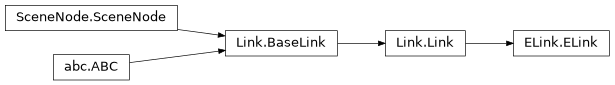
@author: Jesse Haviland

class roboticstoolbox.robot.ELink.ELink(*args, **kwargs)[source]

Bases: Link

A(q=0.0)

Link transform matrix

link.A(q) is an SE(3) matrix that describes the rigid-body transformation from the previous to the current link frame to the next, which depends on the joint coordinate q.

Parameters:: q (float) – Joint coordinate (radians or metres). Not required for links with no variable
Returns:: link frame transformation matrix
Return type:: T

property B: float

Get/set motor viscous friction

link.B is the motor viscous friction
link.B = ... checks and sets the motor viscous friction

Returns:: motor viscous friction
Return type:: B

Notes

Referred to the motor side of the gearbox.
Viscous friction is the same for positive and negative motion.

property G: float

Get/set gear ratio

link.G is the transmission gear ratio
link.G = ... checks and sets the gear ratio

Returns:: gear ratio
Return type:: G

Notes

The ratio of motor motion : link motion
The gear ratio can be negative, see also the flip attribute.

See also

flip()

property I: ndarray

Get/set link inertia

Link inertia is a symmetric 3x3 matrix describing the inertia with respect to a frame with its origin at the centre of mass, and with axes parallel to those of the link frame.

link.I is the link inertia
link.I = ... checks and sets the link inertia

Returns:: link inertia
Return type:: I

Synopsis

The inertia matrix is

$\begin{bmatrix} I_{xx} & I_{xy} & I_{xz} \\ I_{xy} & I_{yy} & I_{yz} \\I_{xz} & I_{yz} & I_{zz} \end{bmatrix}$

and can be specified as either:

a 3 ⨉ 3 symmetric matrix
a 3-vector $(I_{xx}, I_{yy}, I_{zz})$
a 6-vector $(I_{xx}, I_{yy}, I_{zz}, I_{xy}, I_{yz}, I_{xz})$

Notes

Referred to the link side of the gearbox.

property Jm: float

Get/set motor inertia

link.Jm is the motor inertia
link.Jm = ... checks and sets the motor inertia

Returns:: motor inertia
Return type:: Jm

Notes

Referred to the motor side of the gearbox.

property Tc: ndarray

Get/set motor Coulomb friction

link.Tc is the motor Coulomb friction
link.Tc = ... checks and sets the motor Coulomb friction. If a scalar is given the value is set to [T, -T], if a 2-vector it is assumed to be in the order [Tc⁺, Tc⁻]

Coulomb friction is a non-linear friction effect defined by two parameters such that

\[\begin{split}\tau = \left\{ \begin{array}{ll} \tau_C^+ & \mbox{if $\dot{q} > 0$} \\ \tau_C^- & \mbox{if $\dot{q} < 0$} \end{array} \right.\end{split}\]

Returns:: motor Coulomb friction
Return type:: Tc

Notes

Referred to the motor side of the gearbox.
$\tau_C^+$ must be $> 0$, and $\tau_C^-$ must
be $< 0$.

property Ts: Optional[ndarray]

Constant part of link ETS

The ETS for each Link comprises a constant part (possible the identity) followed by an optional joint variable transform. This property returns the constant part. If no constant part is given, this returns an identity matrix.

Returns:: constant part of link transform
Return type:: Ts

Examples

>>> from roboticstoolbox import Link, ET
>>> link = Link( ET.tz(0.333) * ET.Rx(90, 'deg') * ET.Rz() )
>>> link.Ts
array([[ 1.   ,  0.   ,  0.   ,  0.   ],
       [ 0.   ,  0.   , -1.   ,  0.   ],
       [ 0.   ,  1.   ,  0.   ,  0.333],
       [ 0.   ,  0.   ,  0.   ,  1.   ]])
>>> link = Link( ET.Rz() )
>>> link.Ts

__str__()

Pretty prints the ETS Model of the link

Will output angles in degrees

Returns:: pretty print of the robot link
Return type:: str

attach(object)

attach_to(object)

property children: Optional[List[Link]]

List of child links

The list will be empty for a end-effector link

Returns:: child links
Return type:: children

closest_point(shape, inf_dist=1.0, skip=False)

Finds the closest point to a shape

closest_point(shape, inf_dist) returns the minimum euclidean distance between this link and shape, provided it is less than inf_dist. It will also return the points on self and shape in the world frame which connect the line of length distance between the shapes. If the distance is negative then the shapes are collided.

:param : :type : param shape: The shape to compare distance to :param : the shape :type : param inf_dist: The minimum distance within which to consider :param : :type : param skip: Skip setting all shape transforms

Return type:

Tuple[Optional[int], Optional[ndarray], Optional[ndarray]]

Returns:

d – d is the distance between the shapes
p1 – the points in the world frame on the link shape. The points returned are [x, y, z].
p2 – the points in the world frame the shape. The points returned are [x, y, z].

collided(shape, skip=False)

Checks for collision with a shape

iscollided(shape) checks if this link and shape have collided

Parameters:

shape (Shape) – The shape to compare distance to
skip (bool) – Skip setting all shape transforms

Returns:

True if shapes have collided

Return type:

iscollided

property collision: SceneGroup

Get/set joint collision geometry

The collision geometries are what is used to check for collisions.

link.collision is the list of the collision geometries which
represent the collidable shape of the link. :return: the collision geometries :rtype: list of Shape
link.collision = ... checks and sets the collision geometry
link.collision.append(...) add collision geometry

copy()

Copy of link object

link.copy() is a new Link subclass instance with a copy of all the parameters.

Returns:: copy of link object
Return type:: link

dyn(indent=0)

Inertial properties of link as a string

link.dyn() is a string representation the inertial properties of the link object in a multi-line format. The properties shown are mass, centre of mass, inertia, friction, gear ratio and motor properties.

Parameters:: indent – indent each line by this many spaces

:param : :type : type indent: int :param : :type : return: The string representation of the link dynamics :param : :type : rtype: string

Examples

>>> import roboticstoolbox as rtb
>>> robot = rtb.models.DH.Puma560()
>>> print(robot.links[2])        # kinematic parameters
RevoluteDH:   θ=q,  d=0.15005,  a=0.0203,  ⍺=-1.5707963267948966
>>> print(robot.links[2].dyn())  # dynamic parameters
m     =       4.8 
r     =     -0.02   -0.014     0.07 
        |    0.066        0        0 | 
I     = |        0    0.086        0 | 
        |        0        0    0.013 | 
Jm    =    0.0002 
B     =    0.0014 
Tc    =      0.13(+)     -0.1(-) 
G     =       -54 
qlim  =      -2.4 to      2.4

See also

dyntable()

property ets: ETS

Get/set link ets

link.ets is the link ets
link.ets = ... checks and sets the link ets

Parameters:: ets – the new link ets
Returns:: the current link ets
Return type:: ets

friction(qd, coulomb=True)

Compute joint friction

friction(qd) is the joint friction force/torque for joint velocity qd. The friction model includes:

Viscous friction which is a linear function of velocity.
Coulomb friction which is proportional to sign(qd).

\[\begin{split}\tau = G^2 B \dot{q} + |G| \left\{ \begin{array}{ll} \tau_C^+ & \mbox{if $\dot{q} > 0$} \\ \tau_C^- & \mbox{if $\dot{q} < 0$} \end{array} \right.\end{split}\]

Parameters:

qd (float) – The joint velocity
coulomb (bool) – include Coulomb friction

Returns:

the friction force/torque

Return type:

tau

Notes

The friction value should be added to the motor output torque to
determine the nett torque. It has a negative value when qd > 0.
The returned friction value is referred to the output of the
gearbox.
The friction parameters in the Link object are referred to the
motor.
Motor viscous friction is scaled up by $G^2$.
Motor Coulomb friction is scaled up by math:G.
The appropriate Coulomb friction value to use in the
non-symmetric case depends on the sign of the joint velocity, not the motor velocity.
Coulomb friction is zero for zero joint velocity, stiction is
not modeled.
The absolute value of the gear ratio is used. Negative gear
ratios are tricky: the Puma560 robot has negative gear ratio for joints 1 and 3.

property geometry: SceneGroup

Get/set joint visual geometry

link.geometry is the list of the visual geometries which
represent the shape of the link :return: the visual geometries :rtype: list of Shape
link.geometry = ... checks and sets the geometry
link.geometry.append(...) add geometry

property hasdynamics: bool

Link has dynamic parameters (Link superclass)

Link has some assigned (non-default) dynamic parameters. These could have been assigned:

at constructor time, eg. m=1.2
by invoking a setter method, eg. link.m = 1.2

Returns:: Link has dynamic parameters
Return type:: hasdynamics

Examples

>>> import roboticstoolbox as rtb
>>> robot = rtb.models.DH.Puma560()
>>> robot[1].hasdynamics
True

iscollided(shape, skip=False)

Checks for collision with a shape

iscollided(shape) checks if this link and shape have collided

Parameters:

shape (Shape) – The shape to compare distance to
skip (bool) – Skip setting all shape transforms

Returns:

True if shapes have collided

Return type:

iscollided

property isflip: bool

Get/set joint flip

link.flip is the joint flip status
link.flip = ... checks and sets the joint flip status

Joint flip defines the direction of motion of the joint.

flip = False is conventional motion direction:

revolute motion is a positive rotation about the z-axis

prismatic motion is a positive translation along the z-axis

flip = True is the opposite motion direction:

revolute motion is a negative rotation about the z-axis

prismatic motion is a negative translation along the z-axis

Returns:: joint flip
Return type:: isflip

property isjoint: bool

Test if link has joint

The ETS for each Link comprises a constant part (possible the identity) followed by an optional joint variable transform. This property returns the whether the Link contains the variable transform.

Returns:: test if link has a joint
Return type:: isjoint

Examples

>>> from roboticstoolbox import models
>>> robot = models.URDF.Panda()
>>> robot[1].isjoint  # link with joint
True
>>> robot[8].isjoint  # static link
False

islimit(q)

Checks if joint exceeds limit

link.islimit(q) is True if q exceeds the joint limits defined by link.

Parameters:: q (float) – joint coordinate
Returns:: True if joint is exceeded
Return type:: islimit

Notes

If no limits are set always return False.

See also

qlim()

property isprismatic: bool

Checks if the joint is of prismatic type

Returns:

return: True if is prismatic
rtype: bool

property isrevolute: bool

Checks if the joint is of revolute type

Returns:: True if is revolute
Return type:: isrevolute

property jindex: Union[None, int]

Get/set joint index

link.jindex is the joint index
link.jindex = ... checks and sets the joint index

For a serial-link manipulator the joints are numbered starting at zero and increasing sequentially toward the end-effector. For branched mechanisms this is not so straightforward. The link’s jindex property specifies the index of its joint variable within a vector of joint coordinates.

Returns:: joint index
Return type:: jindex

Notes

jindex values must be a sequence of integers starting
at zero.

property m: float

Get/set link mass

link.m is the link mass
link.m = ... checks and sets the link mass

Returns:: link mass
Return type:: m

property name: str

Get/set link name

link.name is the link name
link.name = ... checks and sets the link name

Returns:: link name
Return type:: name

property nchildren: int

Number of child links

Will be zero for an end-effector link

Returns:: number of child links
Return type:: nchildren

nofriction(coulomb=True, viscous=False)

Clone link without friction

link.nofriction() is a copy of the link instance with the same parameters except, the Coulomb and/or viscous friction parameters are set to zero.

Parameters:

coulomb (bool) – if True, will set the Coulomb friction to 0
viscous (bool) – if True, will set the viscous friction to 0

Notes

For simulation it can be useful to remove Couloumb friction
which can cause problems for numerical integration.

property parent: Optional[Self]

Parent link

This is a reference to the links parent in the kinematic chain

Returns:: Link’s parent
Return type:: parent

Examples

>>> from roboticstoolbox import models
>>> robot = models.URDF.Panda()
>>> robot[0].parent  # base link has no parent
>>> robot[1].parent  # second link's parent
Link(name = "panda_link0")

property parent_name: Optional[str]

Parent link name

Returns:: Link’s parent name
Return type:: parent_name

property qlim: Optional[ndarray]

Get/set joint limits

link.qlim is the joint limits
link.qlim = ... checks and sets the joint limits

Returns:: joint limits
Return type:: qlim

Notes

The limits are not widely enforced within the toolbox.
If no joint limits are specified the value is None

See also

islimit()

property r: ndarray

Get/set link centre of mass

The link centre of mass is a 3-vector defined with respect to the link frame.

link.r is the link centre of mass
link.r = ... checks and sets the link centre of mass

Returns:: link centre of mass
Return type:: r

property robot: Optional[BaseRobot]

Get forward reference to the robot which owns this link

link.robot is the robot reference
link.robot = ... checks and sets the robot reference

Returns:: The robot object
Return type:: robot

property scene_children: List[SceneNode]: Returns the child nodes of this object

property scene_parent: Type[SceneNode]: Returns the parent node of this object

property v

Variable part of link ETS

The ETS for each Link comprises a constant part (possible the identity) followed by an optional joint variable transform. This property returns the latter.

Returns:: joint variable transform
Return type:: v

Examples

class roboticstoolbox.robot.ELink.ELink2(*args, **kwargs)[source]

Bases: Link2

A(q=0.0)

Link transform matrix

link.A(q) is an SE(2) matrix that describes the rigid-body transformation from the previous to the current link frame to the next, which depends on the joint coordinate q.

Parameters:: q (float) – Joint coordinate (radians or metres). Not required for links with no variable
Returns:: link frame transformation matrix
Return type:: T

property B: float

Get/set motor viscous friction

link.B is the motor viscous friction
link.B = ... checks and sets the motor viscous friction

Returns:: motor viscous friction
Return type:: B

Notes

Referred to the motor side of the gearbox.
Viscous friction is the same for positive and negative motion.

property G: float

Get/set gear ratio

link.G is the transmission gear ratio
link.G = ... checks and sets the gear ratio

Returns:: gear ratio
Return type:: G

Notes

The ratio of motor motion : link motion
The gear ratio can be negative, see also the flip attribute.

See also

flip()

property I: ndarray

Get/set link inertia

Link inertia is a symmetric 3x3 matrix describing the inertia with respect to a frame with its origin at the centre of mass, and with axes parallel to those of the link frame.

link.I is the link inertia
link.I = ... checks and sets the link inertia

Returns:: link inertia
Return type:: I

Synopsis

The inertia matrix is

$\begin{bmatrix} I_{xx} & I_{xy} & I_{xz} \\ I_{xy} & I_{yy} & I_{yz} \\I_{xz} & I_{yz} & I_{zz} \end{bmatrix}$

and can be specified as either:

a 3 ⨉ 3 symmetric matrix
a 3-vector $(I_{xx}, I_{yy}, I_{zz})$
a 6-vector $(I_{xx}, I_{yy}, I_{zz}, I_{xy}, I_{yz}, I_{xz})$

Notes

Referred to the link side of the gearbox.

property Jm: float

Get/set motor inertia

link.Jm is the motor inertia
link.Jm = ... checks and sets the motor inertia

Returns:: motor inertia
Return type:: Jm

Notes

Referred to the motor side of the gearbox.

property Tc: ndarray

Get/set motor Coulomb friction

link.Tc is the motor Coulomb friction
link.Tc = ... checks and sets the motor Coulomb friction. If a scalar is given the value is set to [T, -T], if a 2-vector it is assumed to be in the order [Tc⁺, Tc⁻]

Coulomb friction is a non-linear friction effect defined by two parameters such that

\[\begin{split}\tau = \left\{ \begin{array}{ll} \tau_C^+ & \mbox{if $\dot{q} > 0$} \\ \tau_C^- & \mbox{if $\dot{q} < 0$} \end{array} \right.\end{split}\]

Returns:: motor Coulomb friction
Return type:: Tc

Notes

Referred to the motor side of the gearbox.
$\tau_C^+$ must be $> 0$, and $\tau_C^-$ must
be $< 0$.

property Ts: Optional[ndarray]

Constant part of link ETS

The ETS for each Link comprises a constant part (possible the identity) followed by an optional joint variable transform. This property returns the constant part. If no constant part is given, this returns an identity matrix.

Returns:: constant part of link transform
Return type:: Ts

Examples

>>> from roboticstoolbox import Link, ET
>>> link = Link( ET.tz(0.333) * ET.Rx(90, 'deg') * ET.Rz() )
>>> link.Ts
array([[ 1.   ,  0.   ,  0.   ,  0.   ],
       [ 0.   ,  0.   , -1.   ,  0.   ],
       [ 0.   ,  1.   ,  0.   ,  0.333],
       [ 0.   ,  0.   ,  0.   ,  1.   ]])
>>> link = Link( ET.Rz() )
>>> link.Ts

__str__()

Pretty prints the ETS Model of the link

Will output angles in degrees

Returns:: pretty print of the robot link
Return type:: str

attach(object)

attach_to(object)

property children: Optional[List[Link]]

List of child links

The list will be empty for a end-effector link

Returns:: child links
Return type:: children

closest_point(shape, inf_dist=1.0, skip=False)

Finds the closest point to a shape

closest_point(shape, inf_dist) returns the minimum euclidean distance between this link and shape, provided it is less than inf_dist. It will also return the points on self and shape in the world frame which connect the line of length distance between the shapes. If the distance is negative then the shapes are collided.

:param : :type : param shape: The shape to compare distance to :param : the shape :type : param inf_dist: The minimum distance within which to consider :param : :type : param skip: Skip setting all shape transforms

Return type:

Tuple[Optional[int], Optional[ndarray], Optional[ndarray]]

Returns:

d – d is the distance between the shapes
p1 – the points in the world frame on the link shape. The points returned are [x, y, z].
p2 – the points in the world frame the shape. The points returned are [x, y, z].

collided(shape, skip=False)

Checks for collision with a shape

iscollided(shape) checks if this link and shape have collided

Parameters:

shape (Shape) – The shape to compare distance to
skip (bool) – Skip setting all shape transforms

Returns:

True if shapes have collided

Return type:

iscollided

property collision: SceneGroup

Get/set joint collision geometry

The collision geometries are what is used to check for collisions.

link.collision is the list of the collision geometries which
represent the collidable shape of the link. :return: the collision geometries :rtype: list of Shape
link.collision = ... checks and sets the collision geometry
link.collision.append(...) add collision geometry

copy()

Copy of link object

link.copy() is a new Link subclass instance with a copy of all the parameters.

Returns:: copy of link object
Return type:: link

dyn(indent=0)

Inertial properties of link as a string

link.dyn() is a string representation the inertial properties of the link object in a multi-line format. The properties shown are mass, centre of mass, inertia, friction, gear ratio and motor properties.

Parameters:: indent – indent each line by this many spaces

:param : :type : type indent: int :param : :type : return: The string representation of the link dynamics :param : :type : rtype: string

Examples

>>> import roboticstoolbox as rtb
>>> robot = rtb.models.DH.Puma560()
>>> print(robot.links[2])        # kinematic parameters
RevoluteDH:   θ=q,  d=0.15005,  a=0.0203,  ⍺=-1.5707963267948966
>>> print(robot.links[2].dyn())  # dynamic parameters
m     =       4.8 
r     =     -0.02   -0.014     0.07 
        |    0.066        0        0 | 
I     = |        0    0.086        0 | 
        |        0        0    0.013 | 
Jm    =    0.0002 
B     =    0.0014 
Tc    =      0.13(+)     -0.1(-) 
G     =       -54 
qlim  =      -2.4 to      2.4

See also

dyntable()

property ets: ETS

Get/set link ets

link.ets is the link ets
link.ets = ... checks and sets the link ets

Parameters:: ets – the new link ets
Returns:: the current link ets
Return type:: ets

friction(qd, coulomb=True)

Compute joint friction

friction(qd) is the joint friction force/torque for joint velocity qd. The friction model includes:

Viscous friction which is a linear function of velocity.
Coulomb friction which is proportional to sign(qd).

\[\begin{split}\tau = G^2 B \dot{q} + |G| \left\{ \begin{array}{ll} \tau_C^+ & \mbox{if $\dot{q} > 0$} \\ \tau_C^- & \mbox{if $\dot{q} < 0$} \end{array} \right.\end{split}\]

Parameters:

qd (float) – The joint velocity
coulomb (bool) – include Coulomb friction

Returns:

the friction force/torque

Return type:

tau

Notes

The friction value should be added to the motor output torque to
determine the nett torque. It has a negative value when qd > 0.
The returned friction value is referred to the output of the
gearbox.
The friction parameters in the Link object are referred to the
motor.
Motor viscous friction is scaled up by $G^2$.
Motor Coulomb friction is scaled up by math:G.
The appropriate Coulomb friction value to use in the
non-symmetric case depends on the sign of the joint velocity, not the motor velocity.
Coulomb friction is zero for zero joint velocity, stiction is
not modeled.
The absolute value of the gear ratio is used. Negative gear
ratios are tricky: the Puma560 robot has negative gear ratio for joints 1 and 3.

property geometry: SceneGroup

Get/set joint visual geometry

link.geometry is the list of the visual geometries which
represent the shape of the link :return: the visual geometries :rtype: list of Shape
link.geometry = ... checks and sets the geometry
link.geometry.append(...) add geometry

property hasdynamics: bool

Link has dynamic parameters (Link superclass)

Link has some assigned (non-default) dynamic parameters. These could have been assigned:

at constructor time, eg. m=1.2
by invoking a setter method, eg. link.m = 1.2

Returns:: Link has dynamic parameters
Return type:: hasdynamics

Examples

>>> import roboticstoolbox as rtb
>>> robot = rtb.models.DH.Puma560()
>>> robot[1].hasdynamics
True

iscollided(shape, skip=False)

Checks for collision with a shape

iscollided(shape) checks if this link and shape have collided

Parameters:

shape (Shape) – The shape to compare distance to
skip (bool) – Skip setting all shape transforms

Returns:

True if shapes have collided

Return type:

iscollided

property isflip: bool

Get/set joint flip

link.flip is the joint flip status
link.flip = ... checks and sets the joint flip status

Joint flip defines the direction of motion of the joint.

flip = False is conventional motion direction:

revolute motion is a positive rotation about the z-axis

prismatic motion is a positive translation along the z-axis

flip = True is the opposite motion direction:

revolute motion is a negative rotation about the z-axis

prismatic motion is a negative translation along the z-axis

Returns:: joint flip
Return type:: isflip

property isjoint: bool

Test if link has joint

The ETS for each Link comprises a constant part (possible the identity) followed by an optional joint variable transform. This property returns the whether the Link contains the variable transform.

Returns:: test if link has a joint
Return type:: isjoint

Examples

>>> from roboticstoolbox import models
>>> robot = models.URDF.Panda()
>>> robot[1].isjoint  # link with joint
True
>>> robot[8].isjoint  # static link
False

islimit(q)

Checks if joint exceeds limit

link.islimit(q) is True if q exceeds the joint limits defined by link.

Parameters:: q (float) – joint coordinate
Returns:: True if joint is exceeded
Return type:: islimit

Notes

If no limits are set always return False.

See also

qlim()

property isprismatic: bool

Checks if the joint is of prismatic type

Returns:

return: True if is prismatic
rtype: bool

property isrevolute: bool

Checks if the joint is of revolute type

Returns:: True if is revolute
Return type:: isrevolute

property jindex: Union[None, int]

Get/set joint index

link.jindex is the joint index
link.jindex = ... checks and sets the joint index

For a serial-link manipulator the joints are numbered starting at zero and increasing sequentially toward the end-effector. For branched mechanisms this is not so straightforward. The link’s jindex property specifies the index of its joint variable within a vector of joint coordinates.

Returns:: joint index
Return type:: jindex

Notes

jindex values must be a sequence of integers starting
at zero.

property m: float

Get/set link mass

link.m is the link mass
link.m = ... checks and sets the link mass

Returns:: link mass
Return type:: m

property name: str

Get/set link name

link.name is the link name
link.name = ... checks and sets the link name

Returns:: link name
Return type:: name

property nchildren: int

Number of child links

Will be zero for an end-effector link

Returns:: number of child links
Return type:: nchildren

nofriction(coulomb=True, viscous=False)

Clone link without friction

link.nofriction() is a copy of the link instance with the same parameters except, the Coulomb and/or viscous friction parameters are set to zero.

Parameters:

coulomb (bool) – if True, will set the Coulomb friction to 0
viscous (bool) – if True, will set the viscous friction to 0

Notes

For simulation it can be useful to remove Couloumb friction
which can cause problems for numerical integration.

property parent: Optional[Self]

Parent link

This is a reference to the links parent in the kinematic chain

Returns:: Link’s parent
Return type:: parent

Examples

>>> from roboticstoolbox import models
>>> robot = models.URDF.Panda()
>>> robot[0].parent  # base link has no parent
>>> robot[1].parent  # second link's parent
Link(name = "panda_link0")

property parent_name: Optional[str]

Parent link name

Returns:: Link’s parent name
Return type:: parent_name

property qlim: Optional[ndarray]

Get/set joint limits

link.qlim is the joint limits
link.qlim = ... checks and sets the joint limits

Returns:: joint limits
Return type:: qlim

Notes

The limits are not widely enforced within the toolbox.
If no joint limits are specified the value is None

See also

islimit()

property r: ndarray

Get/set link centre of mass

The link centre of mass is a 3-vector defined with respect to the link frame.

link.r is the link centre of mass
link.r = ... checks and sets the link centre of mass

Returns:: link centre of mass
Return type:: r

property robot: Optional[BaseRobot]

Get forward reference to the robot which owns this link

link.robot is the robot reference
link.robot = ... checks and sets the robot reference

Returns:: The robot object
Return type:: robot

property scene_children: List[SceneNode]: Returns the child nodes of this object

property scene_parent: Type[SceneNode]: Returns the parent node of this object

property v

Variable part of link ETS

The ETS for each Link comprises a constant part (possible the identity) followed by an optional joint variable transform. This property returns the latter.

Returns:: joint variable transform
Return type:: v

Examples

ERobot models

Defined using ETS

A number of models are defined in terms of elementary transform sequences. They can be listed by:

class roboticstoolbox.models.ETS.Panda[source]

Bases: Robot

Create model of Franka-Emika Panda manipulator

panda = Panda() creates a robot object representing the Franka-Emika Panda robot arm. This robot is represented using the elementary transform sequence (ETS).

ETS taken from [1] based on https://frankaemika.github.io/docs/control_parameters.html

References:

Kinematic Derivatives using the Elementary Transform Sequence, J. Haviland and P. Corke

class roboticstoolbox.models.ETS.Frankie[source]

Bases: Robot

A class representing the Franka Emika Panda robot arm. ETS taken from [1] based on https://frankaemika.github.io/docs/control_parameters.html

Parameters:

et_list (list of etb.robot.et) – List of elementary transforms which represent the robot kinematics
q_idx (list of int) – List of indexes within the ets_list which correspond to joints
name (str, optional) – Name of the robot
manufacturer (str, optional) – Manufacturer of the robot
base (float np.ndarray(4,4), optional) – Location of the base is the world frame
tool (float np.ndarray(4,4), optional) – Offset of the flange of the robot to the end-effector
qz (float np.ndarray(7,)) – The zero joint angle configuration of the robot
qr (float np.ndarray(7,)) – The ready state joint angle configuration of the robot

References: [1] Kinematic Derivatives using the Elementary Transform: Sequence, J. Haviland and P. Corke

class roboticstoolbox.models.ETS.Puma560[source]

Bases: Robot

Create model of Franka-Emika Panda manipulator

puma = Puma560() creates a robot object representing the classic Unimation Puma560 robot arm. This robot is represented using the elementary transform sequence (ETS).

Note

The model has different joint offset conventions compared to DH.Puma560(). For this robot:
- Zero joint angles qz is the vertical configuration, corresponding to qr with DH.Puma560()
- qbent is the bent configuration, corresponding to qz with DH.Puma560()

References:

“A Simple and Systematic Approach to Assigning Denavit–Hartenberg Parameters,”, P. I. Corke, in IEEE Transactions on Robotics, vol. 23, no. 3, pp. 590-594, June 2007, doi: 10.1109/TRO.2007.896765.
https://petercorke.com/robotics/a-simple-and-systematic-approach-to-assigning-denavit-hartenberg-parameters

class roboticstoolbox.models.ETS.Planar_Y[source]

Bases: Robot

Create model of a branched planar manipulator:

L0 -- L1 -+- L2a -- L3a -- EEa
        |
        +- L2b -- L3b -- EEb

Planar_Y() creates a planar branched manipulator model.

References:

Kinematic Derivatives using the Elementary Transform Sequence, J. Haviland and P. Corke

class roboticstoolbox.models.ETS.Planar2[source]

Bases: Robot2

Create model of a branched planar manipulator:

L0 -- L1 -+- L2a -- L3a -- EEa
        |
        +- L2b -- L3b -- EEb

Planar_Y() creates a planar branched manipulator model.

References:

Kinematic Derivatives using the Elementary Transform Sequence, J. Haviland and P. Corke

class roboticstoolbox.models.ETS.GenericSeven[source]

Bases: Robot

Create model of a generic seven degree-of-freedom robot

robot = GenericSeven() creates a robot object. This robot is represented using the elementary transform sequence (ETS).

class roboticstoolbox.models.ETS.XYPanda(workspace=5)[source]

Bases: Robot

Create model of Franka-Emika Panda manipulator on an XY platform

xypanda = XYPanda() creates a robot object representing the Franka-Emika Panda robot arm mounted on an XY platform. This robot is represented using the elementary transform sequence (ETS).

ETS taken from [1] based on https://frankaemika.github.io/docs/control_parameters.html

References:

Kinematic Derivatives using the Elementary Transform Sequence, J. Haviland and P. Corke

Defined from URDF

A number of models are defined in terms of Denavit-Hartenberg parameters, either standard or modified. They can be listed by:

class roboticstoolbox.models.URDF.Panda[source]

Bases: Robot

Class that imports a Panda URDF model

Panda() is a class which imports a Franka-Emika Panda robot definition from a URDF file. The model describes its kinematic and graphical characteristics.

>>> import roboticstoolbox as rtb
>>> robot = rtb.models.URDF.Panda()
>>> print(robot)
ERobot: panda (by Franka Emika), 7 joints (RRRRRRR), 1 gripper, geometry, collision
┌─────┬──────────────┬───────┬─────────────┬────────────────────────────────────────────────┐
│link │     link     │ joint │   parent    │              ETS: parent to link               │
├─────┼──────────────┼───────┼─────────────┼────────────────────────────────────────────────┤
│   0 │ panda_link0  │       │ BASE        │ SE3()                                          │
│   1 │ panda_link1  │     0 │ panda_link0 │ SE3(0, 0, 0.333) ⊕ Rz(q0)                      │
│   2 │ panda_link2  │     1 │ panda_link1 │ SE3(-90°, -0°, 0°) ⊕ Rz(q1)                    │
│   3 │ panda_link3  │     2 │ panda_link2 │ SE3(0, -0.316, 0; 90°, -0°, 0°) ⊕ Rz(q2)       │
│   4 │ panda_link4  │     3 │ panda_link3 │ SE3(0.0825, 0, 0; 90°, -0°, 0°) ⊕ Rz(q3)       │
│   5 │ panda_link5  │     4 │ panda_link4 │ SE3(-0.0825, 0.384, 0; -90°, -0°, 0°) ⊕ Rz(q4) │
│   6 │ panda_link6  │     5 │ panda_link5 │ SE3(90°, -0°, 0°) ⊕ Rz(q5)                     │
│   7 │ panda_link7  │     6 │ panda_link6 │ SE3(0.088, 0, 0; 90°, -0°, 0°) ⊕ Rz(q6)        │
│   8 │ @panda_link8 │       │ panda_link7 │ SE3(0, 0, 0.107)                               │
└─────┴──────────────┴───────┴─────────────┴────────────────────────────────────────────────┘

┌─────┬─────┬────────┬─────┬───────┬─────┬───────┬──────┐
│name │ q0  │ q1     │ q2  │ q3    │ q4  │ q5    │ q6   │
├─────┼─────┼────────┼─────┼───────┼─────┼───────┼──────┤
│  qr │  0° │ -17.2° │  0° │ -126° │  0° │  115° │  45° │
│  qz │  0° │  0°    │  0° │  0°   │  0° │  0°   │  0°  │
└─────┴─────┴────────┴─────┴───────┴─────┴───────┴──────┘

Defined joint configurations are:

qz, zero joint angle configuration, ‘L’ shaped configuration
qr, vertical ‘READY’ configuration
qs, arm is stretched out in the x-direction
qn, arm is at a nominal non-singular configuration

Code author: Jesse Haviland

Section author: Peter Corke

class roboticstoolbox.models.URDF.Frankie[source]

Bases: Robot

Class that imports a Frankie URDF model

Frankie() is a class which imports a Frankie robot definition from a URDF file. The model describes its kinematic and graphical characteristics.

>>> import roboticstoolbox as rtb
>>> robot = rtb.models.URDF.Frankie()
>>> print(robot)
ERobot: frankie (by Franka Emika), 9 joints (RPRRRRRRR), 1 gripper, geometry, collision
┌─────┬────────────────┬───────┬────────────────┬────────────────────────────────────────────────┐
│link │      link      │ joint │     parent     │              ETS: parent to link               │
├─────┼────────────────┼───────┼────────────────┼────────────────────────────────────────────────┤
│   0 │ panda_base0    │       │ BASE           │ SE3()                                          │
│   1 │ panda_base1    │     0 │ panda_base0    │ SE3() ⊕ Rz(q0)                                 │
│   2 │ panda_base_arm │     1 │ panda_base1    │ SE3() ⊕ tx(q1)                                 │
│   3 │ panda_link0    │       │ panda_base_arm │ SE3(0.15, 0, 0.38)                             │
│   4 │ panda_link1    │     2 │ panda_link0    │ SE3(0, 0, 0.333) ⊕ Rz(q2)                      │
│   5 │ panda_link2    │     3 │ panda_link1    │ SE3(-90°, -0°, 0°) ⊕ Rz(q3)                    │
│   6 │ panda_link3    │     4 │ panda_link2    │ SE3(0, -0.316, 0; 90°, -0°, 0°) ⊕ Rz(q4)       │
│   7 │ panda_link4    │     5 │ panda_link3    │ SE3(0.0825, 0, 0; 90°, -0°, 0°) ⊕ Rz(q5)       │
│   8 │ panda_link5    │     6 │ panda_link4    │ SE3(-0.0825, 0.384, 0; -90°, -0°, 0°) ⊕ Rz(q6) │
│   9 │ panda_link6    │     7 │ panda_link5    │ SE3(90°, -0°, 0°) ⊕ Rz(q7)                     │
│  10 │ panda_link7    │     8 │ panda_link6    │ SE3(0.088, 0, 0; 90°, -0°, 0°) ⊕ Rz(q8)        │
│  11 │ @panda_link8   │       │ panda_link7    │ SE3(0, 0, 0.107)                               │
└─────┴────────────────┴───────┴────────────────┴────────────────────────────────────────────────┘

┌─────┬─────┬────┬─────┬────────┬─────┬───────┬─────┬───────┬──────┐
│name │ q0  │ q1 │ q2  │ q3     │ q4  │ q5    │ q6  │ q7    │ q8   │
├─────┼─────┼────┼─────┼────────┼─────┼───────┼─────┼───────┼──────┤
│  qr │  0° │  0 │  0° │ -17.2° │  0° │ -126° │  0° │  115° │  45° │
│  qz │  0° │  0 │  0° │  0°    │  0° │  0°   │  0° │  0°   │  0°  │
└─────┴─────┴────┴─────┴────────┴─────┴───────┴─────┴───────┴──────┘

Defined joint configurations are:

qz, zero joint angle configuration, ‘L’ shaped configuration
qr, vertical ‘READY’ configuration
qs, arm is stretched out in the x-direction
qn, arm is at a nominal non-singular configuration

Code author: Jesse Haviland

Section author: Peter Corke

class roboticstoolbox.models.URDF.FrankieOmni[source]

Bases: Robot

Class that imports an Omnidirectional Frankie URDF model

FrankieOmni() is a class which imports a FrankieOmni robot definition from a URDF file. The model describes its kinematic and graphical characteristics.

>>> import roboticstoolbox as rtb
>>> robot = rtb.models.URDF.FrankieOmni()
>>> print(robot)
ERobot: FrankieOmni (by Custom), 10 joints (PPRRRRRRRR), 1 gripper, 12 branches, dynamics, geometry, collision
┌─────┬────────────────────────┬───────┬───────────────────┬────────────────────────────────────────────────┐
│link │          link          │ joint │      parent       │              ETS: parent to link               │
├─────┼────────────────────────┼───────┼───────────────────┼────────────────────────────────────────────────┤
│   0 │ virtual0               │       │ BASE              │ SE3()                                          │
│   1 │ virtual1               │     0 │ virtual0          │ SE3() ⊕ tx(q0)                                 │
│   2 │ virtual2               │     1 │ virtual1          │ SE3() ⊕ ty(q1)                                 │
│   3 │ base_link              │     2 │ virtual2          │ SE3() ⊕ Rz(q2)                                 │
│   4 │ chassis_link           │       │ base_link         │ SE3()                                          │
│   5 │ left_side_cover_link   │       │ chassis_link      │ SE3()                                          │
│   6 │ right_side_cover_link  │       │ chassis_link      │ SE3()                                          │
│   7 │ front_cover_link       │       │ chassis_link      │ SE3()                                          │
│   8 │ rear_cover_link        │       │ chassis_link      │ SE3()                                          │
│   9 │ front_lights_link      │       │ chassis_link      │ SE3()                                          │
│  10 │ rear_lights_link       │       │ chassis_link      │ SE3()                                          │
│  11 │ top_link               │       │ chassis_link      │ SE3()                                          │
│  12 │ axle_link              │       │ chassis_link      │ SE3(0, 0, 0.05)                                │
│  13 │ front_rocker_link      │       │ axle_link         │ SE3(0.319, 0, 0)                               │
│  14 │ front_left_wheel_link  │       │ front_rocker_link │ SE3(0, 0.2755, 0)                              │
│  15 │ front_right_wheel_link │       │ front_rocker_link │ SE3(0, -0.2755, 0)                             │
│  16 │ rear_rocker_link       │       │ axle_link         │ SE3(-0.319, 0, 0)                              │
│  17 │ rear_left_wheel_link   │       │ rear_rocker_link  │ SE3(0, 0.2755, 0)                              │
│  18 │ rear_right_wheel_link  │       │ rear_rocker_link  │ SE3(0, -0.2755, 0)                             │
│  19 │ base_arm               │       │ base_link         │ tz(0.28)                                       │
│  20 │ panda_link0            │       │ base_arm          │ SE3()                                          │
│  21 │ panda_link1            │     3 │ panda_link0       │ SE3(0, 0, 0.333) ⊕ Rz(q3)                      │
│  22 │ panda_link2            │     4 │ panda_link1       │ SE3(-90°, -0°, 0°) ⊕ Rz(q4)                    │
│  23 │ panda_link3            │     5 │ panda_link2       │ SE3(0, -0.316, 0; 90°, -0°, 0°) ⊕ Rz(q5)       │
│  24 │ panda_link4            │     6 │ panda_link3       │ SE3(0.0825, 0, 0; 90°, -0°, 0°) ⊕ Rz(q6)       │
│  25 │ panda_link5            │     7 │ panda_link4       │ SE3(-0.0825, 0.384, 0; -90°, -0°, 0°) ⊕ Rz(q7) │
│  26 │ panda_link6            │     8 │ panda_link5       │ SE3(90°, -0°, 0°) ⊕ Rz(q8)                     │
│  27 │ panda_link7            │     9 │ panda_link6       │ SE3(0.088, 0, 0; 90°, -0°, 0°) ⊕ Rz(q9)        │
│  28 │ @panda_link8           │       │ panda_link7       │ SE3(0, 0, 0.107)                               │
└─────┴────────────────────────┴───────┴───────────────────┴────────────────────────────────────────────────┘

┌─────┬────┬────┬─────┬─────┬────────┬─────┬───────┬─────┬───────┬──────┐
│name │ q0 │ q1 │ q2  │ q3  │ q4     │ q5  │ q6    │ q7  │ q8    │ q9   │
├─────┼────┼────┼─────┼─────┼────────┼─────┼───────┼─────┼───────┼──────┤
│  qr │  0 │  0 │  0° │  0° │ -17.2° │  0° │ -126° │  0° │  115° │  45° │
│  qz │  0 │  0 │  0° │  0° │  0°    │  0° │  0°   │  0° │  0°   │  0°  │
└─────┴────┴────┴─────┴─────┴────────┴─────┴───────┴─────┴───────┴──────┘

Defined joint configurations are:

qz, zero joint angle configuration, ‘L’ shaped configuration
qr, vertical ‘READY’ configuration
qs, arm is stretched out in the x-direction
qn, arm is at a nominal non-singular configuration

Code author: Jesse Haviland

Section author: Peter Corke

class roboticstoolbox.models.URDF.UR3[source]

Bases: Robot

Class that imports a UR3 URDF model

UR3() is a class which imports a Universal Robotics UR3 robot definition from a URDF file. The model describes its kinematic and graphical characteristics.

>>> import roboticstoolbox as rtb
>>> robot = rtb.models.URDF.UR3()
>>> print(robot)
ERobot: UR3 (by Universal Robotics), 6 joints (RRRRRR), 3 branches, dynamics, geometry, collision
┌─────┬────────────────┬───────┬────────────────┬──────────────────────────────────────────┐
│link │      link      │ joint │     parent     │           ETS: parent to link            │
├─────┼────────────────┼───────┼────────────────┼──────────────────────────────────────────┤
│   0 │ world          │       │ BASE           │ SE3()                                    │
│   1 │ base_link      │       │ world          │ SE3()                                    │
│   2 │ shoulder_link  │     0 │ base_link      │ SE3(0, 0, 0.1519) ⊕ Rz(q0)               │
│   3 │ upper_arm_link │     1 │ shoulder_link  │ SE3(0, 0.1198, 0; 0°, 90°, -0°) ⊕ Ry(q1) │
│   4 │ forearm_link   │     2 │ upper_arm_link │ SE3(0, -0.0925, 0.2437) ⊕ Ry(q2)         │
│   5 │ wrist_1_link   │     3 │ forearm_link   │ SE3(0, 0, 0.2132; 0°, 90°, -0°) ⊕ Ry(q3) │
│   6 │ wrist_2_link   │     4 │ wrist_1_link   │ SE3(0, 0.08505, 0) ⊕ Rz(q4)              │
│   7 │ wrist_3_link   │     5 │ wrist_2_link   │ SE3(0, 0, 0.08535) ⊕ Ry(q5)              │
│   8 │ @ee_link       │       │ wrist_3_link   │ SE3(0, 0.0819, 0; 0°, -0°, 90°)          │
│   9 │ @tool0         │       │ wrist_3_link   │ SE3(0, 0.0819, 0; -90°, -0°, 0°)         │
│  10 │ @base          │       │ base_link      │ SE3(0°, -0°, -180°)                      │
└─────┴────────────────┴───────┴────────────────┴──────────────────────────────────────────┘

┌─────┬───────┬─────┬─────┬─────┬──────┬─────┐
│name │ q0    │ q1  │ q2  │ q3  │ q4   │ q5  │
├─────┼───────┼─────┼─────┼─────┼──────┼─────┤
│  qr │  180° │  0° │  0° │  0° │  90° │  0° │
│  qz │  0°   │  0° │  0° │  0° │  0°  │  0° │
└─────┴───────┴─────┴─────┴─────┴──────┴─────┘

Defined joint configurations are:

qz, zero joint angle configuration, ‘L’ shaped configuration
qr, vertical ‘READY’ configuration

Code author: Jesse Haviland

Section author: Peter Corke

class roboticstoolbox.models.URDF.UR5[source]

Bases: Robot

Class that imports a UR5 URDF model

UR3() is a class which imports a Universal Robotics UR5 robot definition from a URDF file. The model describes its kinematic and graphical characteristics.

>>> import roboticstoolbox as rtb
>>> robot = rtb.models.URDF.UR5()
>>> print(robot)
ERobot: UR5 (by Universal Robotics), 6 joints (RRRRRR), 1 gripper, 3 branches, dynamics, geometry, collision
┌─────┬────────────────┬───────┬────────────────┬──────────────────────────────────────────┐
│link │      link      │ joint │     parent     │           ETS: parent to link            │
├─────┼────────────────┼───────┼────────────────┼──────────────────────────────────────────┤
│   0 │ world          │       │ BASE           │ SE3()                                    │
│   1 │ base_link      │       │ world          │ SE3()                                    │
│   2 │ shoulder_link  │     0 │ base_link      │ SE3(0, 0, 0.08916) ⊕ Rz(q0)              │
│   3 │ upper_arm_link │     1 │ shoulder_link  │ SE3(0, 0.1358, 0; 0°, 90°, -0°) ⊕ Ry(q1) │
│   4 │ forearm_link   │     2 │ upper_arm_link │ SE3(0, -0.1197, 0.425) ⊕ Ry(q2)          │
│   5 │ wrist_1_link   │     3 │ forearm_link   │ SE3(0, 0, 0.3922; 0°, 90°, -0°) ⊕ Ry(q3) │
│   6 │ wrist_2_link   │     4 │ wrist_1_link   │ SE3(0, 0.093, 0) ⊕ Rz(q4)                │
│   7 │ @wrist_3_link  │     5 │ wrist_2_link   │ SE3(0, 0, 0.09465) ⊕ Ry(q5)              │
│   8 │ tool0          │       │ wrist_3_link   │ SE3(0, 0.0823, 0; -90°, -0°, 0°)         │
│   9 │ base           │       │ base_link      │ SE3(0°, -0°, -180°)                      │
└─────┴────────────────┴───────┴────────────────┴──────────────────────────────────────────┘

┌─────┬────────┬────────┬────────┬──────┬────────┬─────┐
│name │ q0     │ q1     │ q2     │ q3   │ q4     │ q5  │
├─────┼────────┼────────┼────────┼──────┼────────┼─────┤
│  qr │  180°  │  0°    │  0°    │  0°  │  90°   │  0° │
│  qz │  0°    │  0°    │  0°    │  0°  │  0°    │  0° │
│  qn │ -40.4° │  20.7° │ -85.6° │  65° │ -40.4° │  0° │
│  q1 │  0°    │ -90°   │  90°   │  0°  │  90°   │  0° │
└─────┴────────┴────────┴────────┴──────┴────────┴─────┘

Defined joint configurations are:

qz, zero joint angle configuration, ‘L’ shaped configuration
qr, vertical ‘READY’ configuration

Code author: Jesse Haviland

Section author: Peter Corke

class roboticstoolbox.models.URDF.UR10[source]

Bases: Robot

Class that imports a UR10 URDF model

UR3() is a class which imports a Universal Robotics UR310 robot definition from a URDF file. The model describes its kinematic and graphical characteristics.

>>> import roboticstoolbox as rtb
>>> robot = rtb.models.URDF.UR10()
>>> print(robot)
ERobot: UR10 (by Universal Robotics), 6 joints (RRRRRR), 3 branches, dynamics, geometry, collision
┌─────┬────────────────┬───────┬────────────────┬──────────────────────────────────────────┐
│link │      link      │ joint │     parent     │           ETS: parent to link            │
├─────┼────────────────┼───────┼────────────────┼──────────────────────────────────────────┤
│   0 │ world          │       │ BASE           │ SE3()                                    │
│   1 │ base_link      │       │ world          │ SE3()                                    │
│   2 │ shoulder_link  │     0 │ base_link      │ SE3(0, 0, 0.1273) ⊕ Rz(q0)               │
│   3 │ upper_arm_link │     1 │ shoulder_link  │ SE3(0, 0.2209, 0; 0°, 90°, -0°) ⊕ Ry(q1) │
│   4 │ forearm_link   │     2 │ upper_arm_link │ SE3(0, -0.1719, 0.612) ⊕ Ry(q2)          │
│   5 │ wrist_1_link   │     3 │ forearm_link   │ SE3(0, 0, 0.5723; 0°, 90°, -0°) ⊕ Ry(q3) │
│   6 │ wrist_2_link   │     4 │ wrist_1_link   │ SE3(0, 0.1149, 0) ⊕ Rz(q4)               │
│   7 │ wrist_3_link   │     5 │ wrist_2_link   │ SE3(0, 0, 0.1157) ⊕ Ry(q5)               │
│   8 │ @ee_link       │       │ wrist_3_link   │ SE3(0, 0.0922, 0; 0°, -0°, 90°)          │
│   9 │ @tool0         │       │ wrist_3_link   │ SE3(0, 0.0922, 0; -90°, -0°, 0°)         │
│  10 │ @base          │       │ base_link      │ SE3(0°, -0°, -180°)                      │
└─────┴────────────────┴───────┴────────────────┴──────────────────────────────────────────┘

┌─────┬───────┬─────┬─────┬─────┬──────┬─────┐
│name │ q0    │ q1  │ q2  │ q3  │ q4   │ q5  │
├─────┼───────┼─────┼─────┼─────┼──────┼─────┤
│  qr │  180° │  0° │  0° │  0° │  90° │  0° │
│  qz │  0°   │  0° │  0° │  0° │  0°  │  0° │
└─────┴───────┴─────┴─────┴─────┴──────┴─────┘

Defined joint configurations are:

qz, zero joint angle configuration, ‘L’ shaped configuration
qr, vertical ‘READY’ configuration

Code author: Jesse Haviland

Section author: Peter Corke

class roboticstoolbox.models.URDF.Puma560[source]

Bases: Robot

Class that imports a Puma 560 URDF model

Puma560() is a class which imports a Unimation Puma560 robot definition from a URDF file. The model describes its kinematic and graphical characteristics.

>>> import roboticstoolbox as rtb
>>> robot = rtb.models.URDF.Puma560()
>>> print(robot)
ERobot: Puma560 (by Unimation), 6 joints (RRRRRR), geometry, collision
┌─────┬────────┬───────┬────────┬───────────────────────────────────────────────────┐
│link │  link  │ joint │ parent │                ETS: parent to link                │
├─────┼────────┼───────┼────────┼───────────────────────────────────────────────────┤
│   0 │ link1  │       │ BASE   │ SE3()                                             │
│   1 │ link2  │     0 │ link1  │ SE3(0, 0, 0.5486; 90°, -0°, 0°) ⊕ Ry(q0)          │
│   2 │ link3  │     1 │ link2  │ SE3(0, 0.07493, 0.1422) ⊕ Rz(q1)                  │
│   3 │ link4  │     2 │ link3  │ SE3(0.4318, 0, 0.0254; 0°, -0°, 90°) ⊕ Rz(q2)     │
│   4 │ link5  │     3 │ link4  │ SE3(0.3518, 0, -0.0381; -90°, -0°, -90°) ⊕ Rz(q3) │
│   5 │ link6  │     4 │ link5  │ SE3(0, 0, 0.0803; 90°, -0°, 0°) ⊕ Rz(q4)          │
│   6 │ @link7 │     5 │ link6  │ SE3(0, 0.05334, 0; -90°, -0°, 0°) ⊕ Rz(q5)        │
└─────┴────────┴───────┴────────┴───────────────────────────────────────────────────┘

┌─────┬───────┬────────┬────────┬────────┬────────┬────────┐
│name │ q0    │ q1     │ q2     │ q3     │ q4     │ q5     │
├─────┼───────┼────────┼────────┼────────┼────────┼────────┤
│  qr │  0°   │  90°   │ -90°   │  0°    │  0°    │  0°    │
│  qz │  0°   │  0°    │  0°    │  0°    │  0°    │  0°    │
│  ru │ -0°   │  45°   │  180°  │ -0°    │  45°   │  0°    │
│  rd │ -0°   │ -47.8° │  5.39° │ -180°  │  47.6° │  180°  │
│  lu │  152° │ -225°  │  5.39° │  145°  │  55.8° │  21.4° │
│  ld │  152° │ -132°  │  180°  │  38.6° │  49.3° │  152°  │
│  qs │  0°   │  0°    │ -90°   │  0°    │  0°    │  0°    │
│  qn │  0°   │  45°   │  180°  │  0°    │  45°   │  0°    │
└─────┴───────┴────────┴────────┴────────┴────────┴────────┘

Defined joint configurations are:

qz, zero joint angle configuration, ‘L’ shaped configuration
qr, vertical ‘READY’ configuration
qs, arm is stretched out in the x-direction
qn, arm is at a nominal non-singular configuration

Warning

This file has been modified so that the zero-angle pose is the same as the DH model in the toolbox. j3 rotation is changed from -𝜋/2 to 𝜋/2. Dimensions are also slightly different. Both models include the pedestal height.

Note

The original file is from https://github.com/nimasarli/puma560_description/blob/master/urdf/puma560_robot.urdf.xacro

Code author: Jesse Haviland

Section author: Peter Corke

class roboticstoolbox.models.URDF.px100[source]

Bases: Robot

Class that imports a PX100 URDF model

px100() is a class which imports an Interbotix px100 robot definition from a URDF file. The model describes its kinematic and graphical characteristics.

>>> import roboticstoolbox as rtb
>>> robot = rtb.models.URDF.px100()
>>> print(robot)
ERobot: px100 (by Interbotix), 7 joints (RRRRRPP), 4 branches, dynamics, geometry, collision
┌─────┬─────────────────────┬───────┬───────────────────┬────────────────────────────────────────────┐
│link │        link         │ joint │      parent       │            ETS: parent to link             │
├─────┼─────────────────────┼───────┼───────────────────┼────────────────────────────────────────────┤
│   0 │ /base_link          │       │ BASE              │ SE3()                                      │
│   1 │ /shoulder_link      │     0 │ /base_link        │ SE3(0, 0, 0.0508) ⊕ Rz(q0)                 │
│   2 │ /upper_arm_link     │     1 │ /shoulder_link    │ SE3(0, 0, 0.04225) ⊕ Ry(q1)                │
│   3 │ /forearm_link       │     2 │ /upper_arm_link   │ SE3(0.035, 0, 0.1; 180°, -0°, 0°) ⊕ Ry(q2) │
│   4 │ /gripper_link       │     3 │ /forearm_link     │ SE3(0.1, 0, 0) ⊕ Ry(q3)                    │
│   5 │ /ee_arm_link        │       │ /gripper_link     │ SE3(0.063, 0, 0; -180°, -0°, 0°)           │
│   6 │ @/gripper_prop_link │     4 │ /ee_arm_link      │ SE3(0.0055, 0, 0) ⊕ Rx(q4)                 │
│   7 │ /gripper_bar_link   │       │ /ee_arm_link      │ SE3()                                      │
│   8 │ /fingers_link       │       │ /gripper_bar_link │ SE3(0.023, 0, 0)                           │
│   9 │ @/left_finger_link  │     5 │ /fingers_link     │ SE3() ⊕ ty(q5)                             │
│  10 │ @/right_finger_link │     6 │ /fingers_link     │ SE3() ⊕ ty(q6)                             │
│  11 │ @/ee_gripper_link   │       │ /fingers_link     │ SE3(0.02757, 0, 0)                         │
└─────┴─────────────────────┴───────┴───────────────────┴────────────────────────────────────────────┘

┌─────┬─────┬────────┬─────┬───────┬─────┬────┬────────┐
│name │ q0  │ q1     │ q2  │ q3    │ q4  │ q5 │ q6     │
├─────┼─────┼────────┼─────┼───────┼─────┼────┼────────┤
│  qr │  0° │ -17.2° │  0° │ -126° │  0° │  2 │  0.785 │
│  qz │  0° │  0°    │  0° │  0°   │  0° │  0 │  0     │
└─────┴─────┴────────┴─────┴───────┴─────┴────┴────────┘

Defined joint configurations are:

qz, zero joint angle configuration, ‘L’ shaped configuration
qr, vertical ‘READY’ configuration

Reference:

https://docs.trossenrobotics.com/interbotix_xsarms_docs/specifications/px100.html

Code author: Jesse Haviland

Section author: Peter Corke

class roboticstoolbox.models.URDF.px150[source]

Bases: Robot

Class that imports a PX150 URDF model

px150() is a class which imports an Interbotix px150 robot definition from a URDF file. The model describes its kinematic and graphical characteristics.

IndexError: index 7 is out of bounds for axis 0 with size 7

Defined joint configurations are:

qz, zero joint angle configuration, ‘L’ shaped configuration
qr, vertical ‘READY’ configuration

Reference:

https://docs.trossenrobotics.com/interbotix_xsarms_docs/specifications/px150.html

Code author: Jesse Haviland

Section author: Peter Corke

class roboticstoolbox.models.URDF.rx150[source]

Bases: Robot

Class that imports a RX150 URDF model

rx150() is a class which imports an Interbotix rx150 robot definition from a URDF file. The model describes its kinematic and graphical characteristics.

IndexError: index 7 is out of bounds for axis 0 with size 7

Defined joint configurations are:

qz, zero joint angle configuration, ‘L’ shaped configuration
qr, vertical ‘READY’ configuration

Reference:

https://docs.trossenrobotics.com/interbotix_xsarms_docs/specifications/rx150.html

Code author: Jesse Haviland

Section author: Peter Corke

class roboticstoolbox.models.URDF.rx200[source]

Bases: Robot

Class that imports a RX200 URDF model

rx200() is a class which imports an Interbotix rx200 robot definition from a URDF file. The model describes its kinematic and graphical characteristics.

IndexError: index 7 is out of bounds for axis 0 with size 7

Defined joint configurations are:

qz, zero joint angle configuration, ‘L’ shaped configuration
qr, vertical ‘READY’ configuration

Reference:

https://docs.trossenrobotics.com/interbotix_xsarms_docs/specifications/rx200.html

Code author: Jesse Haviland

Section author: Peter Corke

class roboticstoolbox.models.URDF.vx300[source]

Bases: Robot

Class that imports a VX300 URDF model

vx300() is a class which imports an Interbotix vx300 robot definition from a URDF file. The model describes its kinematic and graphical characteristics.

>>> import roboticstoolbox as rtb
>>> robot = rtb.models.URDF.vx300()
>>> print(robot)
ERobot: vx300 (by Interbotix), 8 joints (RRRRRRPP), 4 branches, dynamics, geometry, collision
┌─────┬─────────────────────┬───────┬───────────────────┬──────────────────────────────────────────────┐
│link │        link         │ joint │      parent       │             ETS: parent to link              │
├─────┼─────────────────────┼───────┼───────────────────┼──────────────────────────────────────────────┤
│   0 │ /base_link          │       │ BASE              │ SE3()                                        │
│   1 │ /shoulder_link      │     0 │ /base_link        │ SE3(0, 0, 0.0787) ⊕ Rz(q0)                   │
│   2 │ /upper_arm_link     │     1 │ /shoulder_link    │ SE3(0, 0, 0.04805) ⊕ Ry(q1)                  │
│   3 │ /forearm_link       │     2 │ /upper_arm_link   │ SE3(0.05955, 0, 0.3; 180°, -0°, 0°) ⊕ Ry(q2) │
│   4 │ /wrist_link         │     3 │ /forearm_link     │ SE3(0.3, 0, 0) ⊕ Ry(q3)                      │
│   5 │ /gripper_link       │     4 │ /wrist_link       │ SE3(0.06974, 0, 0; -180°, -0°, 0°) ⊕ Rx(q4)  │
│   6 │ /ee_arm_link        │       │ /gripper_link     │ SE3(0.04283, 0, 0)                           │
│   7 │ @/gripper_prop_link │     5 │ /ee_arm_link      │ SE3(0.005675, 0, 0) ⊕ Rx(q5)                 │
│   8 │ /gripper_bar_link   │       │ /ee_arm_link      │ SE3()                                        │
│   9 │ /fingers_link       │       │ /gripper_bar_link │ SE3(0.02587, 0, 0)                           │
│  10 │ @/left_finger_link  │     6 │ /fingers_link     │ SE3() ⊕ ty(q6)                               │
│  11 │ @/right_finger_link │     7 │ /fingers_link     │ SE3() ⊕ ty(q7)                               │
│  12 │ @/ee_gripper_link   │       │ /fingers_link     │ SE3(0.0385, 0, 0)                            │
└─────┴─────────────────────┴───────┴───────────────────┴──────────────────────────────────────────────┘

┌─────┬─────┬────────┬─────┬───────┬─────┬───────┬────────┬────┐
│name │ q0  │ q1     │ q2  │ q3    │ q4  │ q5    │ q6     │ q7 │
├─────┼─────┼────────┼─────┼───────┼─────┼───────┼────────┼────┤
│  qr │  0° │ -17.2° │  0° │ -126° │  0° │  115° │  0.785 │  0 │
│  qz │  0° │  0°    │  0° │  0°   │  0° │  0°   │  0     │  0 │
└─────┴─────┴────────┴─────┴───────┴─────┴───────┴────────┴────┘

Defined joint configurations are:

qz, zero joint angle configuration, ‘L’ shaped configuration
qr, vertical ‘READY’ configuration

Reference:

https://docs.trossenrobotics.com/interbotix_xsarms_docs/specifications/vx300.html

Code author: Jesse Haviland

Section author: Peter Corke

class roboticstoolbox.models.URDF.vx300s[source]

Bases: Robot

Class that imports a VX300s URDF model

vx300s() is a class which imports an Interbotix vx300s robot definition from a URDF file. The model describes its kinematic and graphical characteristics.

>>> import roboticstoolbox as rtb
>>> robot = rtb.models.URDF.vx300s()
>>> print(robot)
ERobot: vx300s (by Interbotix), 9 joints (RRRRRRRPP), 4 branches, dynamics, geometry, collision
┌─────┬─────────────────────┬───────┬─────────────────────┬──────────────────────────────────────────────┐
│link │        link         │ joint │       parent        │             ETS: parent to link              │
├─────┼─────────────────────┼───────┼─────────────────────┼──────────────────────────────────────────────┤
│   0 │ /base_link          │       │ BASE                │ SE3()                                        │
│   1 │ /shoulder_link      │     0 │ /base_link          │ SE3(0, 0, 0.0787) ⊕ Rz(q0)                   │
│   2 │ /upper_arm_link     │     1 │ /shoulder_link      │ SE3(0, 0, 0.04805) ⊕ Ry(q1)                  │
│   3 │ /upper_forearm_link │     2 │ /upper_arm_link     │ SE3(0.05955, 0, 0.3; 180°, -0°, 0°) ⊕ Ry(q2) │
│   4 │ /lower_forearm_link │     3 │ /upper_forearm_link │ SE3(0.2, 0, 0) ⊕ Rx(q3)                      │
│   5 │ /wrist_link         │     4 │ /lower_forearm_link │ SE3(0.1, 0, 0) ⊕ Ry(q4)                      │
│   6 │ /gripper_link       │     5 │ /wrist_link         │ SE3(0.06974, 0, 0; -180°, -0°, 0°) ⊕ Rx(q5)  │
│   7 │ /ee_arm_link        │       │ /gripper_link       │ SE3(0.04283, 0, 0)                           │
│   8 │ @/gripper_prop_link │     6 │ /ee_arm_link        │ SE3(0.005675, 0, 0) ⊕ Rx(q6)                 │
│   9 │ /gripper_bar_link   │       │ /ee_arm_link        │ SE3()                                        │
│  10 │ /fingers_link       │       │ /gripper_bar_link   │ SE3(0.02587, 0, 0)                           │
│  11 │ @/left_finger_link  │     7 │ /fingers_link       │ SE3() ⊕ ty(q7)                               │
│  12 │ @/right_finger_link │     8 │ /fingers_link       │ SE3() ⊕ ty(q8)                               │
│  13 │ @/ee_gripper_link   │       │ /fingers_link       │ SE3(0.0385, 0, 0)                            │
└─────┴─────────────────────┴───────┴─────────────────────┴──────────────────────────────────────────────┘

┌─────┬─────┬────────┬─────┬───────┬─────┬───────┬──────┬────┬────┐
│name │ q0  │ q1     │ q2  │ q3    │ q4  │ q5    │ q6   │ q7 │ q8 │
├─────┼─────┼────────┼─────┼───────┼─────┼───────┼──────┼────┼────┤
│  qr │  0° │ -17.2° │  0° │ -126° │  0° │  115° │  45° │  0 │  0 │
│  qz │  0° │  0°    │  0° │  0°   │  0° │  0°   │  0°  │  0 │  0 │
└─────┴─────┴────────┴─────┴───────┴─────┴───────┴──────┴────┴────┘

Defined joint configurations are:

qz, zero joint angle configuration, ‘L’ shaped configuration
qr, vertical ‘READY’ configuration

Reference:

https://docs.trossenrobotics.com/interbotix_xsarms_docs/specifications/vx300s.html

Code author: Jesse Haviland

Section author: Peter Corke

class roboticstoolbox.models.URDF.wx200[source]

Bases: Robot

Class that imports a WX200 URDF model

wx200() is a class which imports an Interbotix wx200 robot definition from a URDF file. The model describes its kinematic and graphical characteristics.

>>> import roboticstoolbox as rtb
>>> robot = rtb.models.URDF.wx200()
>>> print(robot)
ERobot: wx200 (by Interbotix), 8 joints (RRRRRRPP), 4 branches, dynamics, geometry, collision
┌─────┬─────────────────────┬───────┬───────────────────┬───────────────────────────────────────────┐
│link │        link         │ joint │      parent       │            ETS: parent to link            │
├─────┼─────────────────────┼───────┼───────────────────┼───────────────────────────────────────────┤
│   0 │ /base_link          │       │ BASE              │ SE3()                                     │
│   1 │ /shoulder_link      │     0 │ /base_link        │ SE3(0, 0, 0.0716) ⊕ Rz(q0)                │
│   2 │ /upper_arm_link     │     1 │ /shoulder_link    │ SE3(0, 0, 0.03865) ⊕ Ry(q1)               │
│   3 │ /forearm_link       │     2 │ /upper_arm_link   │ SE3(0.05, 0, 0.2; 180°, -0°, 0°) ⊕ Ry(q2) │
│   4 │ /wrist_link         │     3 │ /forearm_link     │ SE3(0.2, 0, 0) ⊕ Ry(q3)                   │
│   5 │ /gripper_link       │     4 │ /wrist_link       │ SE3(0.065, 0, 0; -180°, -0°, 0°) ⊕ Rx(q4) │
│   6 │ /ee_arm_link        │       │ /gripper_link     │ SE3(0.043, 0, 0)                          │
│   7 │ @/gripper_prop_link │     5 │ /ee_arm_link      │ SE3(0.0055, 0, 0) ⊕ Rx(q5)                │
│   8 │ /gripper_bar_link   │       │ /ee_arm_link      │ SE3()                                     │
│   9 │ /fingers_link       │       │ /gripper_bar_link │ SE3(0.023, 0, 0)                          │
│  10 │ @/left_finger_link  │     6 │ /fingers_link     │ SE3() ⊕ ty(q6)                            │
│  11 │ @/right_finger_link │     7 │ /fingers_link     │ SE3() ⊕ ty(q7)                            │
│  12 │ @/ee_gripper_link   │       │ /fingers_link     │ SE3(0.02757, 0, 0)                        │
└─────┴─────────────────────┴───────┴───────────────────┴───────────────────────────────────────────┘

┌─────┬─────┬────────┬─────┬───────┬─────┬───────┬────────┬────┐
│name │ q0  │ q1     │ q2  │ q3    │ q4  │ q5    │ q6     │ q7 │
├─────┼─────┼────────┼─────┼───────┼─────┼───────┼────────┼────┤
│  qr │  0° │ -17.2° │  0° │ -126° │  0° │  115° │  0.785 │  0 │
│  qz │  0° │  0°    │  0° │  0°   │  0° │  0°   │  0     │  0 │
└─────┴─────┴────────┴─────┴───────┴─────┴───────┴────────┴────┘

Defined joint configurations are:

qz, zero joint angle configuration, ‘L’ shaped configuration
qr, vertical ‘READY’ configuration

Reference:

https://docs.trossenrobotics.com/interbotix_xsarms_docs/specifications/wx200.html

Code author: Jesse Haviland

Section author: Peter Corke

class roboticstoolbox.models.URDF.wx250[source]

Bases: Robot

Class that imports a WX250 URDF model

wx250() is a class which imports an Interbotix wx250 robot definition from a URDF file. The model describes its kinematic and graphical characteristics.

>>> import roboticstoolbox as rtb
>>> robot = rtb.models.URDF.wx250()
>>> print(robot)
ERobot: wx250 (by Interbotix), 8 joints (RRRRRRPP), 4 branches, dynamics, geometry, collision
┌─────┬─────────────────────┬───────┬───────────────────┬───────────────────────────────────────────────┐
│link │        link         │ joint │      parent       │              ETS: parent to link              │
├─────┼─────────────────────┼───────┼───────────────────┼───────────────────────────────────────────────┤
│   0 │ /base_link          │       │ BASE              │ SE3()                                         │
│   1 │ /shoulder_link      │     0 │ /base_link        │ SE3(0, 0, 0.0716) ⊕ Rz(q0)                    │
│   2 │ /upper_arm_link     │     1 │ /shoulder_link    │ SE3(0, 0, 0.03865) ⊕ Ry(q1)                   │
│   3 │ /forearm_link       │     2 │ /upper_arm_link   │ SE3(0.04975, 0, 0.25; 180°, -0°, 0°) ⊕ Ry(q2) │
│   4 │ /wrist_link         │     3 │ /forearm_link     │ SE3(0.25, 0, 0) ⊕ Ry(q3)                      │
│   5 │ /gripper_link       │     4 │ /wrist_link       │ SE3(0.065, 0, 0; -180°, -0°, 0°) ⊕ Rx(q4)     │
│   6 │ /ee_arm_link        │       │ /gripper_link     │ SE3(0.043, 0, 0)                              │
│   7 │ @/gripper_prop_link │     5 │ /ee_arm_link      │ SE3(0.0055, 0, 0) ⊕ Rx(q5)                    │
│   8 │ /gripper_bar_link   │       │ /ee_arm_link      │ SE3()                                         │
│   9 │ /fingers_link       │       │ /gripper_bar_link │ SE3(0.023, 0, 0)                              │
│  10 │ @/left_finger_link  │     6 │ /fingers_link     │ SE3() ⊕ ty(q6)                                │
│  11 │ @/right_finger_link │     7 │ /fingers_link     │ SE3() ⊕ ty(q7)                                │
│  12 │ @/ee_gripper_link   │       │ /fingers_link     │ SE3(0.02757, 0, 0)                            │
└─────┴─────────────────────┴───────┴───────────────────┴───────────────────────────────────────────────┘

┌─────┬─────┬────────┬─────┬───────┬─────┬───────┬────────┬────┐
│name │ q0  │ q1     │ q2  │ q3    │ q4  │ q5    │ q6     │ q7 │
├─────┼─────┼────────┼─────┼───────┼─────┼───────┼────────┼────┤
│  qr │  0° │ -17.2° │  0° │ -126° │  0° │  115° │  0.785 │  0 │
│  qz │  0° │  0°    │  0° │  0°   │  0° │  0°   │  0     │  0 │
└─────┴─────┴────────┴─────┴───────┴─────┴───────┴────────┴────┘

Defined joint configurations are:

qz, zero joint angle configuration, ‘L’ shaped configuration
qr, vertical ‘READY’ configuration

Reference:

https://docs.trossenrobotics.com/interbotix_xsarms_docs/specifications/wx250.html

Code author: Jesse Haviland

Section author: Peter Corke

class roboticstoolbox.models.URDF.wx250s[source]

Bases: Robot

Class that imports a wx250s URDF model

wx250s() is a class which imports an Interbotix wx250s robot definition from a URDF file. The model describes its kinematic and graphical characteristics.

>>> import roboticstoolbox as rtb
>>> robot = rtb.models.URDF.wx250s()
>>> print(robot)
ERobot: wx250s (by Interbotix), 9 joints (RRRRRRRPP), 4 branches, dynamics, geometry, collision
┌─────┬─────────────────────┬───────┬─────────────────────┬───────────────────────────────────────────────┐
│link │        link         │ joint │       parent        │              ETS: parent to link              │
├─────┼─────────────────────┼───────┼─────────────────────┼───────────────────────────────────────────────┤
│   0 │ /base_link          │       │ BASE                │ SE3()                                         │
│   1 │ /shoulder_link      │     0 │ /base_link          │ SE3(0, 0, 0.0716) ⊕ Rz(q0)                    │
│   2 │ /upper_arm_link     │     1 │ /shoulder_link      │ SE3(0, 0, 0.03865) ⊕ Ry(q1)                   │
│   3 │ /upper_forearm_link │     2 │ /upper_arm_link     │ SE3(0.04975, 0, 0.25; 180°, -0°, 0°) ⊕ Ry(q2) │
│   4 │ /lower_forearm_link │     3 │ /upper_forearm_link │ SE3(0.175, 0, 0) ⊕ Rx(q3)                     │
│   5 │ /wrist_link         │     4 │ /lower_forearm_link │ SE3(0.075, 0, 0) ⊕ Ry(q4)                     │
│   6 │ /gripper_link       │     5 │ /wrist_link         │ SE3(0.065, 0, 0; -180°, -0°, 0°) ⊕ Rx(q5)     │
│   7 │ /ee_arm_link        │       │ /gripper_link       │ SE3(0.043, 0, 0)                              │
│   8 │ @/gripper_prop_link │     6 │ /ee_arm_link        │ SE3(0.0055, 0, 0) ⊕ Rx(q6)                    │
│   9 │ /gripper_bar_link   │       │ /ee_arm_link        │ SE3()                                         │
│  10 │ /fingers_link       │       │ /gripper_bar_link   │ SE3(0.023, 0, 0)                              │
│  11 │ @/left_finger_link  │     7 │ /fingers_link       │ SE3() ⊕ ty(q7)                                │
│  12 │ @/right_finger_link │     8 │ /fingers_link       │ SE3() ⊕ ty(q8)                                │
│  13 │ @/ee_gripper_link   │       │ /fingers_link       │ SE3(0.02757, 0, 0)                            │
└─────┴─────────────────────┴───────┴─────────────────────┴───────────────────────────────────────────────┘

┌─────┬─────┬────────┬─────┬───────┬─────┬───────┬──────┬────┬────┐
│name │ q0  │ q1     │ q2  │ q3    │ q4  │ q5    │ q6   │ q7 │ q8 │
├─────┼─────┼────────┼─────┼───────┼─────┼───────┼──────┼────┼────┤
│  qr │  0° │ -17.2° │  0° │ -126° │  0° │  115° │  45° │  0 │  0 │
│  qz │  0° │  0°    │  0° │  0°   │  0° │  0°   │  0°  │  0 │  0 │
└─────┴─────┴────────┴─────┴───────┴─────┴───────┴──────┴────┴────┘

Defined joint configurations are:

qz, zero joint angle configuration, ‘L’ shaped configuration
qr, vertical ‘READY’ configuration

Reference:

https://docs.trossenrobotics.com/interbotix_xsarms_docs/specifications/wx250s.html

Code author: Jesse Haviland

Section author: Peter Corke

class roboticstoolbox.models.URDF.Mico[source]

Bases: Robot

Class that imports a Mico URDF model

Panda() is a class which imports a Kinova Mico robot definition from a URDF file. The model describes its kinematic and graphical characteristics.

>>> import roboticstoolbox as rtb
>>> robot = rtb.models.URDF.Mico()
>>> print(robot)
ERobot: j2n4s300 (by Kinova), 4 joints (RRRR), 1 gripper, dynamics, geometry, collision
┌─────┬────────────────────┬───────┬────────────────────┬────────────────────────────────────────────────────┐
│link │        link        │ joint │       parent       │                ETS: parent to link                 │
├─────┼────────────────────┼───────┼────────────────────┼────────────────────────────────────────────────────┤
│   0 │ world              │       │ BASE               │ SE3()                                              │
│   1 │ root               │       │ world              │ SE3()                                              │
│   2 │ j2n4s300_link_base │       │ root               │ SE3()                                              │
│   3 │ j2n4s300_link_1    │     0 │ j2n4s300_link_base │ SE3(0, 0, 0.1568; 180°, 7.017e-15°, 180°) ⊕ Rz(q0) │
│   4 │ j2n4s300_link_2    │     1 │ j2n4s300_link_1    │ SE3(0, 0.0016, -0.1187; -90°, -0°, 180°) ⊕ Rz(q1)  │
│   5 │ j2n4s300_link_3    │     2 │ j2n4s300_link_2    │ SE3(0, -0.41, 0; 180°, 7.017e-15°, 180°) ⊕ Rz(q2)  │
│   6 │ @j2n4s300_link_4   │     3 │ j2n4s300_link_3    │ SE3(0, 0.2073, -0.0114; -90°, -0°, 180°) ⊕ Rz(q3)  │
└─────┴────────────────────┴───────┴────────────────────┴────────────────────────────────────────────────────┘

┌─────┬─────┬──────┬──────┬─────┐
│name │ q0  │ q1   │ q2   │ q3  │
├─────┼─────┼──────┼──────┼─────┤
│  qr │  0° │  45° │  60° │  0° │
│  qz │  0° │  0°  │  0°  │  0° │
└─────┴─────┴──────┴──────┴─────┘

Defined joint configurations are:

qz, zero joint angle configuration, ‘L’ shaped configuration
qr, vertical ‘READY’ configuration

Code author: Jesse Haviland

Section author: Peter Corke

class roboticstoolbox.models.URDF.PR2[source]: Bases: Robot

class roboticstoolbox.models.URDF.LBR[source]

Bases: Robot

Class that imports a LBR URDF model

LBR() is a class which imports a Franka-Emika LBR robot definition from a URDF file. The model describes its kinematic and graphical characteristics.

>>> import roboticstoolbox as rtb
>>> robot = rtb.models.URDF.LBR()
>>> print(robot)
ERobot: kuka_lbr_iiwa_14_r820 (by Kuka), 7 joints (RRRRRRR), 2 branches, geometry, collision
┌─────┬───────────┬───────┬───────────┬───────────────────────────────────┐
│link │   link    │ joint │  parent   │        ETS: parent to link        │
├─────┼───────────┼───────┼───────────┼───────────────────────────────────┤
│   0 │ base_link │       │ BASE      │ SE3()                             │
│   1 │ link_1    │     0 │ base_link │ SE3() ⊕ Rz(q0)                    │
│   2 │ link_2    │     1 │ link_1    │ SE3(-0.0004362, 0, 0.36) ⊕ Ry(q1) │
│   3 │ link_3    │     2 │ link_2    │ SE3() ⊕ Rz(q2)                    │
│   4 │ link_4    │     3 │ link_3    │ SE3(0.0004362, 0, 0.42) ⊕ Ry(-q3) │
│   5 │ link_5    │     4 │ link_4    │ SE3() ⊕ Rz(q4)                    │
│   6 │ link_6    │     5 │ link_5    │ SE3(0, 0, 0.4) ⊕ Ry(q5)           │
│   7 │ link_7    │     6 │ link_6    │ SE3() ⊕ Rz(q6)                    │
│   8 │ @tool0    │       │ link_7    │ SE3(0, 0, 0.126)                  │
│   9 │ @base     │       │ base_link │ SE3()                             │
└─────┴───────────┴───────┴───────────┴───────────────────────────────────┘

┌─────┬─────┬────────┬─────┬───────┬─────┬────────┬──────┐
│name │ q0  │ q1     │ q2  │ q3    │ q4  │ q5     │ q6   │
├─────┼─────┼────────┼─────┼───────┼─────┼────────┼──────┤
│  qr │  0° │ -17.2° │  0° │ -109° │  0° │  85.9° │  45° │
│  qz │  0° │  0°    │  0° │  0°   │  0° │  0°    │  0°  │
└─────┴─────┴────────┴─────┴───────┴─────┴────────┴──────┘

Defined joint configurations are:

qz, zero joint angle configuration, ‘L’ shaped configuration
qr, vertical ‘READY’ configuration
qs, arm is stretched out in the x-direction
qn, arm is at a nominal non-singular configuration

Code author: Jesse Haviland

Section author: Peter Corke

class roboticstoolbox.models.URDF.KinovaGen3[source]

Bases: Robot

Class that imports a KinovaGen3 URDF model

KinovaGen3() is a class which imports a KinovaGen3 robot definition from a URDF file. The model describes its kinematic and graphical characteristics.

>>> import roboticstoolbox as rtb
>>> robot = rtb.models.URDF.KinovaGen3()
>>> print(robot)
ERobot: gen3 (by Kinova), 7 joints (RRRRRRR), 4 branches, dynamics, geometry, collision
┌─────┬────────────────────────┬───────┬────────────────────────┬────────────────────────────────────────────────────────────────────┐
│link │          link          │ joint │         parent         │                        ETS: parent to link                         │
├─────┼────────────────────────┼───────┼────────────────────────┼────────────────────────────────────────────────────────────────────┤
│   0 │ base_link              │       │ BASE                   │ SE3()                                                              │
│   1 │ shoulder_link          │     0 │ base_link              │ SE3(0, 0, 0.1564; -180°, 1.583e-16°, -2.825e-34°) ⊕ Rz(q0)         │
│   2 │ half_arm_1_link        │     1 │ shoulder_link          │ SE3(0, 0.005375, -0.1284; 90°, 1.223e-15°, -6.361e-15°) ⊕ Rz(q1)   │
│   3 │ half_arm_2_link        │     2 │ half_arm_1_link        │ SE3(0, -0.2104, -0.006375; -90°, 7.062e-31°, -1.669e-14°) ⊕ Rz(q2) │
│   4 │ forearm_link           │     3 │ half_arm_2_link        │ SE3(0, 0.006375, -0.2104; 90°, -3.836e-15°, -9.541e-15°) ⊕ Rz(q3)  │
│   5 │ spherical_wrist_1_link │     4 │ forearm_link           │ SE3(0, -0.2084, -0.006375; -90°, 1.272e-14°, -3.651e-15°) ⊕ Rz(q4) │
│   6 │ spherical_wrist_2_link │     5 │ spherical_wrist_1_link │ SE3(0, 0.000175, -0.1059; 90°, 5.276e-26°, -4.707e-13°) ⊕ Rz(q5)   │
│   7 │ bracelet_link          │     6 │ spherical_wrist_2_link │ SE3(0, -0.1059, -0.000175; -90°, -3.181e-15°, 5.523e-15°) ⊕ Rz(q6) │
│   8 │ end_effector_link      │       │ bracelet_link          │ SE3(0, 0, -0.06153; 180°, 6.299e-31°, 0°)                          │
│   9 │ @camera_link           │       │ end_effector_link      │ SE3(0, 0.05639, -0.00305; -1.851e-13°, 1.851e-13°, 180°)           │
│  10 │ @camera_depth_frame    │       │ end_effector_link      │ SE3(0.0275, 0.066, -0.00305; -1.851e-13°, 1.851e-13°, 180°)        │
│  11 │ @camera_color_frame    │       │ end_effector_link      │ SE3(0, 0.05639, -0.00305; -1.851e-13°, 1.851e-13°, 180°)           │
│  12 │ @tool_frame            │       │ end_effector_link      │ SE3()                                                              │
└─────┴────────────────────────┴───────┴────────────────────────┴────────────────────────────────────────────────────────────────────┘

┌─────┬───────┬────────┬─────┬────────┬─────┬────────┬──────┐
│name │ q0    │ q1     │ q2  │ q3     │ q4  │ q5     │ q6   │
├─────┼───────┼────────┼─────┼────────┼─────┼────────┼──────┤
│  qr │  180° │ -17.2° │  0° │ -91.7° │  0° │ -57.3° │  90° │
│  qz │  0°   │  0°    │  0° │  0°    │  0° │  0°    │  0°  │
└─────┴───────┴────────┴─────┴────────┴─────┴────────┴──────┘

Defined joint configurations are:

qz, zero joint angle configuration, ‘L’ shaped configuration
qr, vertical ‘READY’ configuration
qs, arm is stretched out in the x-direction
qn, arm is at a nominal non-singular configuration

Code author: Jesse Haviland

Section author: Peter Corke

class roboticstoolbox.models.URDF.YuMi[source]

Bases: Robot

Class that imports an ABB YuMi URDF model

YuMi() is a class which imports an ABB YuMi (IRB14000) robot definition from a URDF file. The model describes its kinematic and graphical characteristics.

>>> import roboticstoolbox as rtb
>>> robot = rtb.models.URDF.YuMi()
>>> print(robot)
ERobot: yumi (by ABB), 14 joints (RRRRRRRRRRRRRR), 2 grippers, 2 branches, dynamics, geometry, collision
┌─────┬─────────────────┬───────┬────────────────┬───────────────────────────────────────────────────────────────────┐
│link │      link       │ joint │     parent     │                        ETS: parent to link                        │
├─────┼─────────────────┼───────┼────────────────┼───────────────────────────────────────────────────────────────────┤
│   0 │ world           │       │ BASE           │ SE3()                                                             │
│   1 │ yumi_base_link  │       │ world          │ SE3(0, 0, 0.1)                                                    │
│   2 │ yumi_body       │       │ yumi_base_link │ SE3()                                                             │
│   3 │ yumi_link_1_r   │     0 │ yumi_body      │ SE3(0.05355, -0.0725, 0.4149; -56.12°, -32.56°, -132.7°) ⊕ Rz(q0) │
│   4 │ yumi_link_2_r   │     1 │ yumi_link_1_r  │ SE3(0.03, 0, 0.1; 90°, -0°, 0°) ⊕ Rz(q1)                          │
│   5 │ yumi_link_3_r   │     2 │ yumi_link_2_r  │ SE3(-0.03, 0.1728, 0; -90°, -0°, 0°) ⊕ Rz(q2)                     │
│   6 │ yumi_link_4_r   │     3 │ yumi_link_3_r  │ SE3(-0.04188, 0, 0.07873; 0°, -90°, 90°) ⊕ Rz(q3)                 │
│   7 │ yumi_link_5_r   │     4 │ yumi_link_4_r  │ SE3(0.0405, 0.1646, 0; -90°, -0°, 0°) ⊕ Rz(q4)                    │
│   8 │ yumi_link_6_r   │     5 │ yumi_link_5_r  │ SE3(-0.027, 0, 0.1004; 90°, -0°, 0°) ⊕ Rz(q5)                     │
│   9 │ yumi_link_7_r   │     6 │ yumi_link_6_r  │ SE3(0.027, 0.029, 0; -90°, -0°, 0°) ⊕ Rz(q6)                      │
│  10 │ @gripper_r_base │       │ yumi_link_7_r  │ SE3(0, 0, 0.007; 0°, -0°, -180°)                                  │
│  11 │ yumi_link_1_l   │     7 │ yumi_body      │ SE3(0.05355, 0.0725, 0.4149; 56.04°, -32.75°, 132.8°) ⊕ Rz(q7)    │
│  12 │ yumi_link_2_l   │     8 │ yumi_link_1_l  │ SE3(0.03, 0, 0.1; 90°, -0°, 0°) ⊕ Rz(q8)                          │
│  13 │ yumi_link_3_l   │     9 │ yumi_link_2_l  │ SE3(-0.03, 0.1728, 0; -90°, -0°, 0°) ⊕ Rz(q9)                     │
│  14 │ yumi_link_4_l   │    10 │ yumi_link_3_l  │ SE3(-0.04188, 0, 0.07873; 0°, -90°, 90°) ⊕ Rz(q10)                │
│  15 │ yumi_link_5_l   │    11 │ yumi_link_4_l  │ SE3(0.0405, 0.1646, 0; -90°, -0°, 0°) ⊕ Rz(q11)                   │
│  16 │ yumi_link_6_l   │    12 │ yumi_link_5_l  │ SE3(-0.027, 0, 0.1004; 90°, -0°, 0°) ⊕ Rz(q12)                    │
│  17 │ yumi_link_7_l   │    13 │ yumi_link_6_l  │ SE3(0.027, 0.029, 0; -90°, -0°, 0°) ⊕ Rz(q13)                     │
│  18 │ @gripper_l_base │       │ yumi_link_7_l  │ SE3(0, 0, 0.007; 0°, -0°, -180°)                                  │
└─────┴─────────────────┴───────┴────────────────┴───────────────────────────────────────────────────────────────────┘

┌─────┬─────┬────────┬─────┬───────┬─────┬───────┬──────┬─────┬────────┬─────┬───────┬─────┬───────┬──────┐
│name │ q0  │ q1     │ q2  │ q3    │ q4  │ q5    │ q6   │ q7  │ q8     │ q9  │ q10   │ q11 │ q12   │ q13  │
├─────┼─────┼────────┼─────┼───────┼─────┼───────┼──────┼─────┼────────┼─────┼───────┼─────┼───────┼──────┤
│  qr │  0° │ -17.2° │  0° │ -126° │  0° │  115° │  45° │  0° │ -17.2° │  0° │ -126° │  0° │  115° │  45° │
│  qz │  0° │  0°    │  0° │  0°   │  0° │  0°   │  0°  │  0° │  0°    │  0° │  0°   │  0° │  0°   │  0°  │
│  q1 │  0° │ -22.9° │  0° │  0°   │  0° │  0°   │  0°  │  0° │ -22.9° │  0° │  0°   │  0° │  0°   │  0°  │
└─────┴─────┴────────┴─────┴───────┴─────┴───────┴──────┴─────┴────────┴─────┴───────┴─────┴───────┴──────┘

Defined joint configurations are:

qz, zero joint angle configuration, ‘L’ shaped configuration
qr, vertical ‘READY’ configuration

Reference:

https://github.com/OrebroUniversity/yumi

Code author: Jesse Haviland

Section author: Peter Corke

class roboticstoolbox.models.URDF.Fetch[source]

Bases: Robot

Class that imports a Fetch URDF model

Fetch() is a class which imports a Fetch robot definition from a URDF file. The model describes its kinematic and graphical characteristics.

>>> import roboticstoolbox as rtb
>>> robot = rtb.models.URDF.Fetch()
>>> print(robot)
ERobot: fetch (by Fetch), 10 joints (RPPRRRRRRR), 1 gripper, 6 branches, dynamics, geometry, collision
┌─────┬────────────────────┬───────┬────────────────────┬─────────────────────────────────────────────────────────┐
│link │        link        │ joint │       parent       │                   ETS: parent to link                   │
├─────┼────────────────────┼───────┼────────────────────┼─────────────────────────────────────────────────────────┤
│   0 │ base0              │       │ BASE               │ SE3()                                                   │
│   1 │ base1              │     0 │ base0              │ SE3() ⊕ Rz(q0)                                          │
│   2 │ base_link          │     1 │ base1              │ SE3() ⊕ tx(q1)                                          │
│   3 │ torso_lift_link    │     2 │ base_link          │ SE3(-0.08687, 0, 0.3774; -3.508e-15°, -0°, 0°) ⊕ tz(q2) │
│   4 │ shoulder_pan_link  │     3 │ torso_lift_link    │ SE3(0.1195, 0, 0.3486) ⊕ Rz(q3)                         │
│   5 │ shoulder_lift_link │     4 │ shoulder_pan_link  │ SE3(0.117, 0, 0.06) ⊕ Ry(q4)                            │
│   6 │ upperarm_roll_link │     5 │ shoulder_lift_link │ SE3(0.219, 0, 0) ⊕ Rx(q5)                               │
│   7 │ elbow_flex_link    │     6 │ upperarm_roll_link │ SE3(0.133, 0, 0) ⊕ Ry(q6)                               │
│   8 │ forearm_roll_link  │     7 │ elbow_flex_link    │ SE3(0.197, 0, 0) ⊕ Rx(q7)                               │
│   9 │ wrist_flex_link    │     8 │ forearm_roll_link  │ SE3(0.1245, 0, 0) ⊕ Ry(q8)                              │
│  10 │ @wrist_roll_link   │     9 │ wrist_flex_link    │ SE3(0.1385, 0, 0) ⊕ Rx(q9)                              │
│  11 │ bellows_link       │       │ torso_lift_link    │ SE3()                                                   │
│  12 │ bellows_link2      │       │ torso_lift_link    │ SE3()                                                   │
│  13 │ estop_link         │       │ base_link          │ SE3(-0.1246, 0.2389, 0.3113; 90°, -0°, 0°)              │
│  14 │ laser_link         │       │ base_link          │ SE3(0.235, 0, 0.2878; -180°, -0°, 0°)                   │
│  15 │ torso_fixed_link   │       │ base_link          │ SE3(-0.08687, 0, 0.3774; -3.508e-15°, -0°, 0°)          │
└─────┴────────────────────┴───────┴────────────────────┴─────────────────────────────────────────────────────────┘

┌─────┬─────┬────┬───────┬────────┬────────┬────────┬────────┬─────┬────────┬─────┐
│name │ q0  │ q1 │ q2    │ q3     │ q4     │ q5     │ q6     │ q7  │ q8     │ q9  │
├─────┼─────┼────┼───────┼────────┼────────┼────────┼────────┼─────┼────────┼─────┤
│  qr │  0° │  0 │  0.05 │  75.6° │  80.2° │ -11.5° │  98.5° │  0° │  95.1° │  0° │
│  qz │  0° │  0 │  0    │  0°    │  0°    │  0°    │  0°    │  0° │  0°    │  0° │
└─────┴─────┴────┴───────┴────────┴────────┴────────┴────────┴─────┴────────┴─────┘

Defined joint configurations are:

qz, zero joint angle configuration, arm is stretched out in the x-direction
qr, tucked arm configuration

Code author: Kerry He

Section author: Peter Corke

class roboticstoolbox.models.URDF.FetchCamera[source]

Bases: Robot

Class that imports a FetchCamera URDF model

FetchCamera() is a class which imports a FetchCamera robot definition from a URDF file. The model describes its kinematic and graphical characteristics.

>>> import roboticstoolbox as rtb
>>> robot = rtb.models.URDF.Fetch()
>>> print(robot)
ERobot: fetch (by Fetch), 10 joints (RPPRRRRRRR), 1 gripper, 6 branches, dynamics, geometry, collision
┌─────┬────────────────────┬───────┬────────────────────┬─────────────────────────────────────────────────────────┐
│link │        link        │ joint │       parent       │                   ETS: parent to link                   │
├─────┼────────────────────┼───────┼────────────────────┼─────────────────────────────────────────────────────────┤
│   0 │ base0              │       │ BASE               │ SE3()                                                   │
│   1 │ base1              │     0 │ base0              │ SE3() ⊕ Rz(q0)                                          │
│   2 │ base_link          │     1 │ base1              │ SE3() ⊕ tx(q1)                                          │
│   3 │ torso_lift_link    │     2 │ base_link          │ SE3(-0.08687, 0, 0.3774; -3.508e-15°, -0°, 0°) ⊕ tz(q2) │
│   4 │ shoulder_pan_link  │     3 │ torso_lift_link    │ SE3(0.1195, 0, 0.3486) ⊕ Rz(q3)                         │
│   5 │ shoulder_lift_link │     4 │ shoulder_pan_link  │ SE3(0.117, 0, 0.06) ⊕ Ry(q4)                            │
│   6 │ upperarm_roll_link │     5 │ shoulder_lift_link │ SE3(0.219, 0, 0) ⊕ Rx(q5)                               │
│   7 │ elbow_flex_link    │     6 │ upperarm_roll_link │ SE3(0.133, 0, 0) ⊕ Ry(q6)                               │
│   8 │ forearm_roll_link  │     7 │ elbow_flex_link    │ SE3(0.197, 0, 0) ⊕ Rx(q7)                               │
│   9 │ wrist_flex_link    │     8 │ forearm_roll_link  │ SE3(0.1245, 0, 0) ⊕ Ry(q8)                              │
│  10 │ @wrist_roll_link   │     9 │ wrist_flex_link    │ SE3(0.1385, 0, 0) ⊕ Rx(q9)                              │
│  11 │ bellows_link       │       │ torso_lift_link    │ SE3()                                                   │
│  12 │ bellows_link2      │       │ torso_lift_link    │ SE3()                                                   │
│  13 │ estop_link         │       │ base_link          │ SE3(-0.1246, 0.2389, 0.3113; 90°, -0°, 0°)              │
│  14 │ laser_link         │       │ base_link          │ SE3(0.235, 0, 0.2878; -180°, -0°, 0°)                   │
│  15 │ torso_fixed_link   │       │ base_link          │ SE3(-0.08687, 0, 0.3774; -3.508e-15°, -0°, 0°)          │
└─────┴────────────────────┴───────┴────────────────────┴─────────────────────────────────────────────────────────┘

┌─────┬─────┬────┬───────┬────────┬────────┬────────┬────────┬─────┬────────┬─────┐
│name │ q0  │ q1 │ q2    │ q3     │ q4     │ q5     │ q6     │ q7  │ q8     │ q9  │
├─────┼─────┼────┼───────┼────────┼────────┼────────┼────────┼─────┼────────┼─────┤
│  qr │  0° │  0 │  0.05 │  75.6° │  80.2° │ -11.5° │  98.5° │  0° │  95.1° │  0° │
│  qz │  0° │  0 │  0    │  0°    │  0°    │  0°    │  0°    │  0° │  0°    │  0° │
└─────┴─────┴────┴───────┴────────┴────────┴────────┴────────┴─────┴────────┴─────┘

Defined joint configurations are:

qz, zero joint angle configuration
qr, zero joint angle configuration

Code author: Kerry He

Section author: Peter Corke

class roboticstoolbox.models.URDF.Valkyrie(variant='A')[source]

Bases: Robot

Class that imports a NASA Valkyrie URDF model

Valkyrie() is a class which imports a NASA Valkyrie robot definition from a URDF file. The model describes its kinematic and graphical characteristics.

>>> import roboticstoolbox as rtb
>>> robot = rtb.models.URDF.Valkyrie()
>>> print(robot)
ERobot: valkyrie (by NASA), 58 joints (RRRRRRRRRRRRRRRRRRRRRRRRRRRRRRRRRRRRRRRRRRRRRRRRRRRRRRRRRR), 18 branches, dynamics, geometry, collision
┌─────┬──────────────────────────────┬───────┬─────────────────────────────┬──────────────────────────────────────────────────────────┐
│link │             link             │ joint │           parent            │                   ETS: parent to link                    │
├─────┼──────────────────────────────┼───────┼─────────────────────────────┼──────────────────────────────────────────────────────────┤
│   0 │ pelvis                       │       │ BASE                        │ SE3()                                                    │
│   1 │ torsoYawLink                 │     0 │ pelvis                      │ SE3() ⊕ Rz(q0)                                           │
│   2 │ torsoPitchLink               │     1 │ torsoYawLink                │ SE3(0.04191, 0, 0) ⊕ Ry(q1)                              │
│   3 │ torso                        │     2 │ torsoPitchLink              │ SE3(0, 0, 0.0203) ⊕ Rx(q2)                               │
│   4 │ lowerNeckPitchLink           │     3 │ torso                       │ SE3(0.02035, 0, 0.3384) ⊕ Ry(q3)                         │
│   5 │ neckYawLink                  │     4 │ lowerNeckPitchLink          │ SE3(-0.05192, 0, 0) ⊕ Rz(q4)                             │
│   6 │ upperNeckPitchLink           │     5 │ neckYawLink                 │ SE3(-0.06, 0, 0.196) ⊕ Ry(q5)                            │
│   7 │ @multisense_root_link        │       │ upperNeckPitchLink          │ SE3(0.1836, 0, 0.07535; -180°, 7.5°, 0°)                 │
│   8 │ rightShoulderPitchLink       │     6 │ torso                       │ SE3(-0.0316, 0, 0.2984) ⊕ Ry(q6)                         │
│   9 │ rightShoulderRollLink        │     7 │ rightShoulderPitchLink      │ SE3(0, -0.2499, 0) ⊕ Rx(q7)                              │
│  10 │ rightShoulderYawLink         │     8 │ rightShoulderRollLink       │ SE3() ⊕ Ry(q8)                                           │
│  11 │ rightElbowPitchLink          │     9 │ rightShoulderYawLink        │ SE3(0.0254, -0.33, 0) ⊕ Rz(q9)                           │
│  12 │ rightForearmLink             │    10 │ rightElbowPitchLink         │ SE3(-0.0254, 0, 0) ⊕ Ry(q10)                             │
│  13 │ rightWristRollLink           │    11 │ rightForearmLink            │ SE3(0, -0.2871, 0) ⊕ Rx(q11)                             │
│  14 │ rightPalm                    │    12 │ rightWristRollLink          │ SE3() ⊕ Rz(q12)                                          │
│  15 │ rightThumbRollLink           │    13 │ rightPalm                   │ SE3(0.0049, -0.0351, 0.0228; 20°, -0°, 0°) ⊕ Ry(q13)     │
│  16 │ rightThumbPitch1Link         │    14 │ rightThumbRollLink          │ SE3(0, 0, 0.0229; -20°, -0°, 0°) ⊕ Rx(q14)               │
│  17 │ rightThumbPitch2Link         │    15 │ rightThumbPitch1Link        │ SE3(0, -0.0066, 0.0375) ⊕ Rx(q15)                        │
│  18 │ @rightThumbPitch3Link        │    16 │ rightThumbPitch2Link        │ SE3(0, -0.0049, 0.0275) ⊕ Rx(q16)                        │
│  19 │ rightIndexFingerPitch1Link   │    17 │ rightPalm                   │ SE3(0.0022, -0.0976, 0.0235; -9.998°, -0°, 0°) ⊕ Rz(q17) │
│  20 │ rightIndexFingerPitch2Link   │    18 │ rightIndexFingerPitch1Link  │ SE3(0, -0.0381, 0) ⊕ Rz(q18)                             │
│  21 │ @rightIndexFingerPitch3Link  │    19 │ rightIndexFingerPitch2Link  │ SE3(0, -0.0229, 0) ⊕ Rz(q19)                             │
│  22 │ rightMiddleFingerPitch1Link  │    20 │ rightPalm                   │ SE3(0.0022, -0.097, -0.0119; 7.002°, -0°, 0°) ⊕ Rz(q20)  │
│  23 │ rightMiddleFingerPitch2Link  │    21 │ rightMiddleFingerPitch1Link │ SE3(0, -0.0381, 0) ⊕ Rz(q21)                             │
│  24 │ @rightMiddleFingerPitch3Link │    22 │ rightMiddleFingerPitch2Link │ SE3(0, -0.0229, 0) ⊕ Rz(q22)                             │
│  25 │ rightPinkyPitch1Link         │    23 │ rightPalm                   │ SE3(0.0022, -0.0838, -0.041; 7.002°, -0°, 0°) ⊕ Rz(q23)  │
│  26 │ rightPinkyPitch2Link         │    24 │ rightPinkyPitch1Link        │ SE3(0, -0.0381, 0) ⊕ Rz(q24)                             │
│  27 │ @rightPinkyPitch3Link        │    25 │ rightPinkyPitch2Link        │ SE3(0, -0.0229, 0) ⊕ Rz(q25)                             │
│  28 │ leftShoulderPitchLink        │    26 │ torso                       │ SE3(-0.0316, 0, 0.2984) ⊕ Ry(q26)                        │
│  29 │ leftShoulderRollLink         │    27 │ leftShoulderPitchLink       │ SE3(0, 0.2499, 0) ⊕ Rx(q27)                              │
│  30 │ leftShoulderYawLink          │    28 │ leftShoulderRollLink        │ SE3() ⊕ Ry(q28)                                          │
│  31 │ leftElbowPitchLink           │    29 │ leftShoulderYawLink         │ SE3(0.0254, 0.33, 0) ⊕ Rz(q29)                           │
│  32 │ leftForearmLink              │    30 │ leftElbowPitchLink          │ SE3(-0.0254, 0, 0) ⊕ Ry(q30)                             │
│  33 │ leftWristRollLink            │    31 │ leftForearmLink             │ SE3(0, 0.2871, 0) ⊕ Rx(q31)                              │
│  34 │ leftPalm                     │    32 │ leftWristRollLink           │ SE3() ⊕ Rz(q32)                                          │
│  35 │ leftThumbRollLink            │    33 │ leftPalm                    │ SE3(0.0049, 0.0351, 0.0228; -20°, -0°, 0°) ⊕ Ry(q33)     │
│  36 │ leftThumbPitch1Link          │    34 │ leftThumbRollLink           │ SE3(0, 0, 0.0229; 20°, -0°, 0°) ⊕ Rx(q34)                │
│  37 │ leftThumbPitch2Link          │    35 │ leftThumbPitch1Link         │ SE3(0, 0.0066, 0.0375) ⊕ Rx(q35)                         │
│  38 │ @leftThumbPitch3Link         │    36 │ leftThumbPitch2Link         │ SE3(0, 0.0049, 0.0275) ⊕ Rx(q36)                         │
│  39 │ leftIndexFingerPitch1Link    │    37 │ leftPalm                    │ SE3(0.0022, 0.0976, 0.0235; 9.998°, -0°, 0°) ⊕ Rz(q37)   │
│  40 │ leftIndexFingerPitch2Link    │    38 │ leftIndexFingerPitch1Link   │ SE3(0, 0.0381, 0) ⊕ Rz(q38)                              │
│  41 │ @leftIndexFingerPitch3Link   │    39 │ leftIndexFingerPitch2Link   │ SE3(0, 0.0229, 0) ⊕ Rz(q39)                              │
│  42 │ leftMiddleFingerPitch1Link   │    40 │ leftPalm                    │ SE3(0.0022, 0.097, -0.0119; -7.002°, -0°, 0°) ⊕ Rz(q40)  │
│  43 │ leftMiddleFingerPitch2Link   │    41 │ leftMiddleFingerPitch1Link  │ SE3(0, 0.0381, 0) ⊕ Rz(q41)                              │
│  44 │ @leftMiddleFingerPitch3Link  │    42 │ leftMiddleFingerPitch2Link  │ SE3(0, 0.0229, 0) ⊕ Rz(q42)                              │
│  45 │ leftPinkyPitch1Link          │    43 │ leftPalm                    │ SE3(0.0022, 0.0838, -0.041; -7.002°, -0°, 0°) ⊕ Rz(q43)  │
│  46 │ leftPinkyPitch2Link          │    44 │ leftPinkyPitch1Link         │ SE3(0, 0.0381, 0) ⊕ Rz(q44)                              │
│  47 │ @leftPinkyPitch3Link         │    45 │ leftPinkyPitch2Link         │ SE3(0, 0.0229, 0) ⊕ Rz(q45)                              │
│  48 │ @leftTorsoImu_Frame          │       │ torso                       │ SE3(-0.06276, 0.1342, 0.3631; -89.99°, -0°, 0°)          │
│  49 │ @rightHazardCamera_Frame     │       │ torso                       │ SE3(0.0345, -0.0406, 0.1135; 89.95°, -0°, 89.95°)        │
│  50 │ @leftHazardCamera_Frame      │       │ torso                       │ SE3(0.0345, 0.0406, 0.1135; 89.95°, -0°, 89.95°)         │
│  51 │ rightHipYawLink              │    46 │ pelvis                      │ SE3(0, -0.1016, -0.1853) ⊕ Rz(q46)                       │
│  52 │ rightHipRollLink             │    47 │ rightHipYawLink             │ SE3() ⊕ Rx(q47)                                          │
│  53 │ rightHipPitchLink            │    48 │ rightHipRollLink            │ SE3(0, 0, -0.0609) ⊕ Ry(q48)                             │
│  54 │ rightKneePitchLink           │    49 │ rightHipPitchLink           │ SE3(0.0001122, -0.0361, -0.431) ⊕ Ry(q49)                │
│  55 │ rightAnklePitchLink          │    50 │ rightKneePitchLink          │ SE3(-0.01024, 0, -0.4063) ⊕ Ry(q50)                      │
│  56 │ rightFoot                    │    51 │ rightAnklePitchLink         │ SE3() ⊕ Rx(q51)                                          │
│  57 │ @rightCOP_Frame              │       │ rightFoot                   │ SE3(0.0189, 0, -0.0783)                                  │
│  58 │ @rightFootSixAxis_Frame      │       │ rightFoot                   │ SE3(0.02156, 0, -0.05105; 179.9°, -0°, 0°)               │
│  59 │ leftHipYawLink               │    52 │ pelvis                      │ SE3(0, 0.1016, -0.1853) ⊕ Rz(q52)                        │
│  60 │ leftHipRollLink              │    53 │ leftHipYawLink              │ SE3() ⊕ Rx(q53)                                          │
│  61 │ leftHipPitchLink             │    54 │ leftHipRollLink             │ SE3(0, 0, -0.0609) ⊕ Ry(q54)                             │
│  62 │ leftKneePitchLink            │    55 │ leftHipPitchLink            │ SE3(0.0001122, 0.0361, -0.431) ⊕ Ry(q55)                 │
│  63 │ leftAnklePitchLink           │    56 │ leftKneePitchLink           │ SE3(-0.01024, 0, -0.4063) ⊕ Ry(q56)                      │
│  64 │ leftFoot                     │    57 │ leftAnklePitchLink          │ SE3() ⊕ Rx(q57)                                          │
│  65 │ @leftCOP_Frame               │       │ leftFoot                    │ SE3(0.0189, 0, -0.0783)                                  │
│  66 │ @leftFootSixAxis_Frame       │       │ leftFoot                    │ SE3(0.02156, 0, -0.05105; 179.9°, -0°, 0°)               │
│  67 │ @pelvisRearImu_Frame         │       │ pelvis                      │ SE3(-0.07584, 0, -0.1111; -180°, 27.3°, -180°)           │
│  68 │ @pelvisMiddleImu_Frame       │       │ pelvis                      │ SE3(0, 0, -0.1082; 180°, -0°, 0°)                        │
└─────┴──────────────────────────────┴───────┴─────────────────────────────┴──────────────────────────────────────────────────────────┘

Defined joint configurations are:

qz, zero joint angle configuration, ‘L’ shaped configuration
qr, vertical ‘READY’ configuration

Reference:

https://github.com/gkjohnson/nasa-urdf-robots

Code author: Peter Corke

class roboticstoolbox.models.URDF.AL5D[source]

Bases: Robot

Class that imports a AL5D URDF model

AL5D() is a class which imports a Lynxmotion AL5D robot definition from a URDF file. The model describes its kinematic and graphical characteristics.

>>> import roboticstoolbox as rtb
>>> robot = rtb.models.URDF.AL5D()
>>> print(robot)
ERobot: AL5D (by Lynxmotion), 4 joints (RRRR), dynamics, geometry
┌─────┬────────┬───────┬────────┬─────────────────────────────────────────────────────┐
│link │  link  │ joint │ parent │                 ETS: parent to link                 │
├─────┼────────┼───────┼────────┼─────────────────────────────────────────────────────┤
│   0 │ base   │       │ BASE   │ SE3()                                               │
│   1 │ link1  │     0 │ base   │ SE3(0, 0, 0.06858; 180°, 3.379e-08°, 180°) ⊕ Rz(q0) │
│   2 │ link2  │     1 │ link1  │ SE3(0.002, 0, 0; 0°, 90°, -90°) ⊕ Rz(q1)            │
│   3 │ link3  │     2 │ link2  │ SE3(0.1468, 0, 0; 180°, 3.379e-08°, -90°) ⊕ Rz(q2)  │
│   4 │ @link4 │     3 │ link3  │ SE3(0.1775, 0, 0; 180°, -0°, 90°) ⊕ Rz(q3)          │
└─────┴────────┴───────┴────────┴─────────────────────────────────────────────────────┘

┌─────┬─────┬─────┬──────┬─────┐
│name │ q0  │ q1  │ q2   │ q3  │
├─────┼─────┼─────┼──────┼─────┤
│  qz │  0° │  0° │  0°  │  0° │
│  up │  0° │  0° │  90° │  0° │
└─────┴─────┴─────┴──────┴─────┘

Defined joint configurations are:

qz, zero joint angle configuration, ‘L’ shaped configuration
up, robot poiting upwards

Code author: Tassos Natsakis