Kernel.DoG

classmethod Kernel.DoG(sigma1, sigma2=None, h=None)

Difference of Gaussians kernel

Parameters:

• sigma1 (float) – standard deviation of first Gaussian kernel

• sigma2 (float, optional) – standard deviation of second Gaussian kernel

• h (int, optional) – half-width of Gaussian kernel

Returns:

2h+1 x 2h+1 kernel

Return type:

Kernel

Return the 2-dimensional difference of Gaussian kernel defined by two standard deviation values:

\[\mathbf{K} = G(\sigma_1) - G(\sigma_2)\]

where \(\sigma_1 > \sigma_2\). By default, \(\sigma_2 = 1.6 \sigma_1\).

The kernel is centred within a square array with side length given by:

• \(2 \mbox{ceil}(3 \sigma) + 1\), or

• \(2\mathtt{h} + 1\)

Example:

>>> from machinevisiontoolbox import Kernel
>>> K = Kernel.DoG(1)
>>> K
Kernel: 7x7, min=-0.094, max=0.012, mean=-3.1e-19, SYMMETRIC (DoG σ1=1, σ2=1.6)
>>> K.print()
  0.00  0.00  0.01  0.01  0.01  0.00  0.00
  0.00  0.01  0.01  0.01  0.01  0.01  0.00
  0.01  0.01 -0.01 -0.04 -0.01  0.01  0.01
  0.01  0.01 -0.04 -0.09 -0.04  0.01  0.01
  0.01  0.01 -0.01 -0.04 -0.01  0.01  0.01
  0.00  0.01  0.01  0.01  0.01  0.01  0.00
  0.00  0.00  0.01  0.01  0.01  0.00  0.00

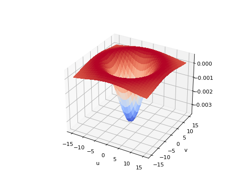
Example:

>>> Kernel.DoG(5, 15).disp3d()

(Source code, png, hires.png, pdf)

Note

• This kernel is similar to the Laplacian of Gaussian and is often used as an efficient approximation.

• This is a “Mexican hat” shaped kernel

References:

• P. Corke, Robotics, Vision & Control for Python, Springer, 2023, Section 11.5.1.3.

Seealso:

LoG Gauss