Robot manipulator blocks

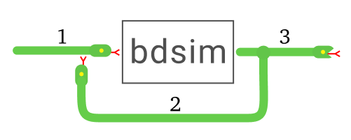
class roboticstoolbox.blocks.arm.FKine(*args: Any, **kwargs: Any)

Bases: FunctionBlock

FKINE

Robot arm forward kinematics.

Inputs:

1

Outputs:

1

States:

0

Port type	Port number	Types	Description
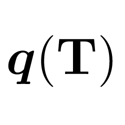
Input	0	ndarray(N)	\(\mathit{q}\)
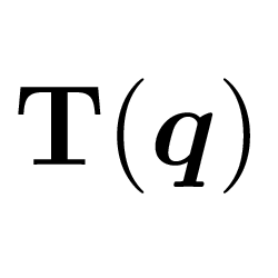
Output	0	SE3	\(\mathbf{T}\)

Compute the end-effector pose as an SE(3) object as a function of the input joint configuration.

Seealso:

fkine()

__init__(robot=None, args={}, **blockargs)

Parameters:

• *inputs (Block or Plug) – Optional incoming connections

• robot (Robot subclass, optional) – Robot model, defaults to None

• args (dict, optional) – Options for fkine, defaults to {}

• blockargs (dict) – common Block options

class roboticstoolbox.blocks.arm.IKine(*args: Any, **kwargs: Any)

Bases: FunctionBlock

IKINE

Robot arm inverse kinematics.

Inputs:

1

Outputs:

1

States:

0

Port type	Port number	Types	Description
Input	0	SE3	\(\mathbf{T}\)
Output	0	ndarray(N)	\(\mathit{q}\)

Compute joint configuration required to achieve end-effector pose input as an SE(3) object.

Note:

The solution may not exist and is not unique. The solution will depend on the initial joint configuration q0.

Seealso:

ik_LM()

__init__(robot=None, q0=None, useprevious=True, ik=None, args={}, seed=None, **blockargs)

Parameters:

• robot (Robot subclass, optional) – Robot model, defaults to None

• q0 (array_like(n), optional) – Initial joint angles, defaults to None

• useprevious (bool, optional) – Use previous IK solution as q0, defaults to True

• ik (str) – Specify an IK function, defaults to “LM”

• args (dict) – Options passed to IK function

• seed (int) – random seed for solution

• blockargs (dict) – common Block options

class roboticstoolbox.blocks.arm.Jacobian(*args: Any, **kwargs: Any)

Bases: FunctionBlock

JACOBIAN

Robot arm Jacobian matrix.

Inputs:

1

Outputs:

1

States:

0

Port type	Port number	Types	Description
Input	0	ndarray(N)	\(\mathit{q}\)
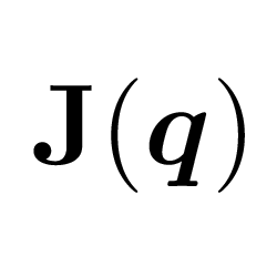
Output	0	ndarray(N,N)	\(\mathbf{J}\)

Compute the Jacobian matrix as a function of the input joint configuration. The Jacobian can be computed in the world or end-effector frame, for spatial or analytical velocity, and its inverse, damped inverse or transpose can be returned.

Seealso:

jacob0() jacobe() jacob0_analytical()

__init__(robot, frame='0', representation=None, inverse=False, pinv=False, damping=None, transpose=False, **blockargs)

Parameters:

• robot (Robot subclass) – Robot model

• frame (str, optional) – Frame to compute Jacobian for, one of: “0” [default], “e”

• representation (str, optional) – representation for analytical Jacobian

• inverse (bool, optional) – output inverse of Jacobian, defaults to False

• pinv (bool, optional) – output pseudo-inverse of Jacobian, defaults to False

• damping (float or array_like(N)) – damping term for inverse, defaults to None

• transpose (bool, optional) – output transpose of Jacobian, defaults to False

• blockargs (dict) – common Block options

If an inverse is requested and damping is not None it is added to the diagonal of the Jacobian prior to the inversion. If a scalar is provided it is added to each element of the diagonal, otherwise an N-vector is assumed.

Note

• Only one of inverse or pinv can be True

• inverse or pinv can be used in conjunction with transpose

• inverse requires that the Jacobian is square

• If inverse is True and the Jacobian is singular a runtime error will occur.

class roboticstoolbox.blocks.arm.ArmPlot(*args: Any, **kwargs: Any)

Bases: GraphicsBlock

ARMPLOT

Plot robot arm.

Inputs:

1 [ndarray(N)]

Outputs:

0

States:

0

Inputs:

1

Outputs:

0

States:

0

Port type	Port number	Types	Description
Input	0	ndarray(N)	\(\mathit{q}\), joint configuration

Create a robot animation using the robot’s plot method.

Seealso:

plot()

PLOT3D = True

__init__(robot=None, q0=None, backend=None, **blockargs)

Parameters:

• robot (Robot subclass) – Robot model

• q0 (ndarray(N)) – initial joint angles, defaults to None

• backend (str, optional) – RTB backend name, defaults to ‘pyplot’

• blockargs (dict) – common GraphicsBlock options

class roboticstoolbox.blocks.arm.JTraj(*args: Any, **kwargs: Any)

Bases: SourceBlock

JTRAJ

Joint-space trajectory

Inputs:

0

Outputs:

3

States:

0

Port type	Port number	Types	Description
Output	0	ndarray	\(q(s)\)
Output	1	ndarray	\(\dot{q}(s)\)
Output	2	ndarray	\(\ddot{q}(s)\)

Outputs a joint space trajectory where the joint coordinates vary from q0 to qf over the course of the simulation. A quintic (5th order) polynomial is used with default zero boundary conditions for velocity and acceleration.

Seealso:

ctraj() xplot() jtraj()

__init__(q0, qf, qd0=None, qdf=None, T=None, **blockargs)

Parameters:

• q0 (array_like(n)) – initial joint coordinate

• qf (array_like(n)) – final joint coordinate

• T (array_like or int, optional) – time vector or number of steps, defaults to None

• qd0 (array_like(n), optional) – initial velocity, defaults to None

• qdf (array_like(n), optional) – final velocity, defaults to None

• blockargs (dict) – common Block options

class roboticstoolbox.blocks.arm.CTraj(*args: Any, **kwargs: Any)

Bases: SourceBlock

CTRAJ

Task space trajectory

Inputs:

0

Outputs:

1

States:

0

Port type	Port number	Types	Description
Output	0	SE3	\(\mathbf{T}(t)\)

The block outputs a pose that varies smoothly from T1 to T2 over the course of T seconds.

If T is not given it defaults to the simulation time.

If trapezoidal is True then a trapezoidal motion profile is used along the path to provide initial acceleration and final deceleration. Otherwise, motion is at constant velocity.

Seealso:

interp() ctraj() xplot() jtraj()

__init__(T1, T2, T, trapezoidal=True, **blockargs)

Parameters:

• T1 (SE3) – initial pose

• T2 (SE3) – final pose

• T (float) – motion time

• trapezoidal (bool) – Use LSPB motion profile along the path

• blockargs (dict) – common Block options

class roboticstoolbox.blocks.arm.CirclePath(radius=1, centre=(0, 0, 0), pose=None, frequency=1, unit='rps', phase=None, **blockargs)

Bases: SourceBlock

CIRCLEPATH

Circular motion.

Inputs:

0 or 1

Outputs:

1

States:

0

Port type	Port number	Types	Description
Output	0	ndarray(3) or SE3	\(\mathit{p}(t)\) or \(\mathbf{T}(t)\)

The block outputs the coordinates of a point moving in a circle of radius r centred at centre and parallel to the xy-plane.

By default the output is a 3-vector \((x, y, z)\) but if pose is an SE3 instance the output is a copy of that pose with its translation set to the coordinate of the moving point. This is the motion of a frame with fixed orientation following a circular path.

__init__(radius=1, centre=(0, 0, 0), pose=None, frequency=1, unit='rps', phase=None, **blockargs)

Parameters:

• radius (float) – radius of circle, defaults to 1

• centre (array_like(3)) – center of circle, defaults to [0,0,0]

• pose (SE3) – SE3 pose of output, defaults to None

• frequency (float) – rotational frequency, defaults to 1

• unit (str) – unit for frequency, one of: ‘rps’ [default], ‘rad’

• phase (float | None) – phase

• blockargs (dict) – common Block options

class roboticstoolbox.blocks.arm.Trapezoidal(*args: Any, **kwargs: Any)

Bases: SourceBlock

Trapezoidal

Trapezoidal scalar trajectory

Inputs:

0

Outputs:

3

States:

0

Port type	Port number	Types	Description
Output	0	float	\(q(t)\)
Output	1	float	\(\dot{q}(t)\)
Output	2	float	\(\ddot{q}(t)\)

Scalar trapezoidal trajectory that varies from q0 to qf over the simulation period.

Seealso:

ctraj(), qplot(), jtraj()

__init__(q0, qf, V=None, T=None, **blockargs)

Compute a joint-space trajectory

Parameters:

• q0 (float) – initial joint coordinate

• qf (float) – final joint coordinate

• T (float, optional) – maximum time, defaults to None

• blockargs (dict) – common Block options

If T is given the value qf is reached at this time. This can be less or greater than the simulation time.

class roboticstoolbox.blocks.arm.Traj(*args: Any, **kwargs: Any)

Bases: FunctionBlock

TRAJ

Vector trajectory

Inputs:

0 or 1

Outputs:

3

States:

0

Port type	Port number	Types	Description
Input	0	float	\(s \in [0, 1]\) distance along trajectory.
Output	0	ndarray	\(y(s)\)
Output	1	ndarray	\(\dot{y}(s)\)
Output	2	ndarray	\(\ddot{y}(s)\)

Generates a vector trajectory using a trapezoidal or quintic polynomial profile that varies from y0 to yf

The distance along the trajectory is either:

• a linear function from 0 to T or maximum simulation time if time is True, or

• the value [0, 1] given on inport port if time is False

Seealso:

spatialmath.base.mtraj()

__init__(y0=0, yf=1, T=None, time=False, traj='trapezoidal', **blockargs)

Parameters:

• y0 (array_like(m), optional) – initial value, defaults to 0

• yf (array_like(m), optional) – final value, defaults to 1

• T (float, optional) – maximum time, defaults to None

• time (bool, optional) – if True trajectory is based on simulation time, else based on input 0. Defaults to False

• traj (str, optional) – trajectory type, one of: ‘trapezoidal’ [default], ‘quintic’

• blockargs (dict) – common Block options

class roboticstoolbox.blocks.arm.IDyn(*args: Any, **kwargs: Any)

Bases: FunctionBlock

IDYN

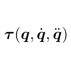
Robot arm forward dynamics model.

Inputs:

3

Outputs:

1

States:

0

Port type	Port number	Types	Description
Input	0	ndarray(N)	\(\mathit{q}\), joint configuration
Input	1	ndarray(N)	\(\dot{\mathit{q}}\), joint velocity
Input	2	ndarray(N)	\(\ddot{\mathit{q}}\), joint acceleration
Output	0	ndarray(N)	\(\mathit{Q}\), generalized joint force

Compute the generalized joint torques required to achieve the input joint configuration, velocity and acceleration. This uses the recursive Newton-Euler (RNE) algorithm.

Seealso:

rne()

__init__(robot, gravity=None, **blockargs)

Parameters:

• robot (Robot subclass) – Robot model

• gravity (ndarray(3)) – gravitational acceleration in the world frame, downwards gravitational force is equivalent to robot base acceleration upwards (positive)

• blockargs (dict) – common Block options

class roboticstoolbox.blocks.arm.Gravload(*args: Any, **kwargs: Any)

Bases: FunctionBlock

GRAVLOAD

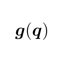
Robot arm gravity load.

Inputs:

1

Outputs:

1

States:

0

Port type	Port number	Types	Description
Input	0	ndarray(N)	\(\mathit{q}\), joint configuration
Output	0	ndarray(N)	\(\mathit{g}\), generalized joint force

Compute generalized joint forces due to gravity for the input joint configuration.

Seealso:

gravload()

__init__(robot, gravity=None, **blockargs)

Parameters:

• robot (Robot subclass) – Robot model

• gravity (ndarray(3)) – gravitational acceleration in the world frame, downwards gravitational force is equivalent to robot base acceleration upwards (positive)

• blockargs (dict) – common Block options

class roboticstoolbox.blocks.arm.Gravload_X(*args: Any, **kwargs: Any)

Bases: FunctionBlock

GRAVLOAD_X

Task-space robot arm gravity wrench.

Inputs:

1

Outputs:

1

States:

0

Port type	Port number	Types	Description
Input	0	ndarray(6)	\(\mathit{x}\), end-effector pose
Output	0	ndarray(6)	\(\mathit{g}_x\), generalized joint force

Compute end-effector wrench due to gravity for the input end-effector pose.

Seealso:

gravload_x() gravload()

__init__(robot, representation='rpy/xyz', gravity=None, **blockargs)

Parameters:

• robot (Robot subclass) – Robot model

• representation (str) – task-space representation, defaults to “rpy/xyz”

• gravity (ndarray(3)) – gravitational acceleration in the world frame, downwards gravitational force is equivalent to robot base acceleration upwards (positive)

• blockargs (dict) – common Block options

class roboticstoolbox.blocks.arm.Inertia(*args: Any, **kwargs: Any)

Bases: FunctionBlock

INERTIA

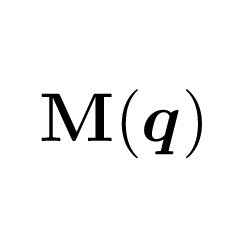
Robot arm inertia matrix.

Inputs:

1 [ndarray(N)]

Outputs:

3 [ndarray(N,N)]

States:

0

Inputs:

1

Outputs:

1

States:

0

Port type	Port number	Types	Description
Input	0	ndarray	\(\mathit{q}\), joint configuration
Output	0	ndarray(N,N)	\(\mathbf{M}\), mass matrix

Joint-space inertia matrix (mass matrix) as a function of joint configuration.

Seealso:

inertia()

__init__(robot, **blockargs)

Parameters:

• robot (Robot subclass) – Robot model

• blockargs (dict) – common Block options

class roboticstoolbox.blocks.arm.Inertia_X(*args: Any, **kwargs: Any)

Bases: FunctionBlock

INERTIA_X

Task-space robot arm inertia matrix.

Inputs:

1

Outputs:

1

States:

0

Port type	Port number	Types	Description
Input	0	ndarray(6)	\(\mathit{x}\), end-effector pose
Output	0	ndarray(6,6)	\(\mathbf{M_x}\), task-space mass matrix

Task-space inertia matrix as a function of end-effector pose.

Seealso:

inertia_x()

__init__(robot, representation='rpy/xyz', pinv=False, **blockargs)

Parameters:

• robot (Robot subclass) – Robot model

• representation (str) – task-space representation, defaults to “rpy/xyz”

• blockargs (dict) – common Block options

class roboticstoolbox.blocks.arm.FDyn(*args: Any, **kwargs: Any)

Bases: ContinuousBlock

FDYN

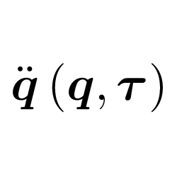
Robot arm forward dynamics.

Inputs:

1

Outputs:

3

States:

2N

Port type	Port number	Types	Description
Input	0	ndarray(N)	\(\mathit{Q}\), generalized joint force
Output	0	ndarray(N)	\(\mathit{q}\), joint configuration
Output	1	ndarray(N)	\(\dot{\mathit{q}}\), joint velocity
Output	2	ndarray(N)	\(\ddot{\mathit{q}}\), joint acceleration

Compute the manipulator arm forward dynamics in joint space, the joint acceleration for the input configuration and applied joint forces. The acceleration is integrated to obtain joint velocity and joint configuration.

Seealso:

fdyn()

__init__(robot, q0=None, **blockargs)

Parameters:

• robot (Robot subclass) – Robot model

• q0 (array_like(n)) – Initial joint configuration

• blockargs (dict) – common Block options

class roboticstoolbox.blocks.arm.FDyn_X(*args: Any, **kwargs: Any)

Bases: ContinuousBlock

FDYN_X

Task-space robot arm forward dynamics.

Inputs:

1

Outputs:

3

States:

12

Port type	Port number	Types	Description
Input	0	ndarray(6)	\(\mathit{\tau}\), end-effector wrench
Output	0	ndarray(6)	\(\mathit{x}\), end-effector pose
Output	1	ndarray(6)	\(\dot{\mathit{x}}\), end-effector velocity
Output	2	ndarray(6)	\(\dot{\mathit{x}}`\), end-effector acceleration

Compute the manipulator arm forward dynamics in task space, the end-effector acceleration for the input end-effector pose and applied end-effector wrench. The acceleration is integrated to obtain task-space velocity and task-space pose.

Seealso:

fdyn_x()

__init__(robot, q0=None, gravcomp=False, velcomp=False, representation='rpy/xyz', **blockargs)

Parameters:

• robot (Robot subclass) – Robot model

• q0 (array_like(n)) – Initial joint configuration

• gravcomp (bool) – perform gravity compensation

• velcomp (bool) – perform velocity term compensation

• representation (str) – task-space representation, defaults to “rpy/xyz”

• blockargs (dict) – common Block options