Kernel.HGauss

classmethod Kernel.HGauss(sigma, h=None)

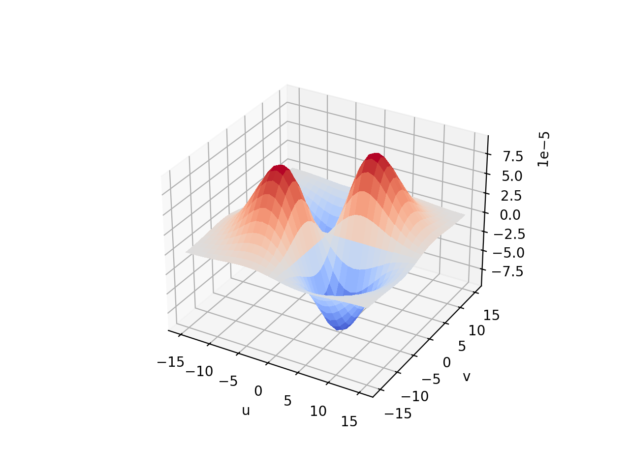
Hessian of Gaussian kernel

Parameters:

• sigma (float) – standard deviation of Gaussian kernel

• h (int, optional) – half-width of kernel

Returns:

2h+1 x 2h+1 kernels: Hxx, Hyy, Hxy

Return type:

(Kernel, Kernel, Kernel)

Returns the Hessian of Gaussian with standard deviation sigma as three 2-dimensional kernels

\[\begin{split}\mathbf{K}_{xx} &= \frac{x^2 - \sigma^2}{2\pi \sigma^3} e^{-(x^2 + y^2) / 2 \sigma^2} \\ \mathbf{K}_{yy} &= \frac{y^2 - \sigma^2}{2\pi \sigma^3} e^{-(x^2 + y^2) / 2 \sigma^2} \\ \mathbf{K}_{xy} &= \frac{xy}{2\pi \sigma^6} e^{-(x^2 + y^2) / 2 \sigma^2}\end{split}\]

The second derivative of an image \(\bf{I}\) at point \((x,y)\) is given by:

\[\begin{split}\begin{bmatrix} (\bf{K}_{xx} * \bf{I})_{x,y} & (\bf{K}_{xy} * \bf{I})_{x,y} \\ (\bf{K}_{xy} * \bf{I})_{x,y} & (\bf{K}_{yy} * \bf{I})_{x,y} \end{bmatrix}\end{split}\]

This second derivative matrix is the Gaussian curvature of the image at \((x,y)\).

The kernels are centred within a square array with side length given by:

• \(2 \mbox{ceil}(3 \sigma) + 1\), or

• \(2\mathtt{h} + 1\)

Example:

>>> from machinevisiontoolbox import Kernel
>>> Hxx, Hyy, Hxy = Kernel.HGauss(1)
>>> Hxx
Kernel: 7x7, min=-0.16, max=0.065, mean=-8.3e-05 (Hxx σ=1)
>>> Hxx.print()
  0.00  0.00  0.00 -0.00  0.00  0.00  0.00
  0.00  0.01  0.00 -0.02  0.00  0.01  0.00
  0.01  0.04  0.00 -0.10  0.00  0.04  0.01
  0.01  0.06  0.00 -0.16  0.00  0.06  0.01
  0.01  0.04  0.00 -0.10  0.00  0.04  0.01
  0.00  0.01  0.00 -0.02  0.00  0.01  0.00
  0.00  0.00  0.00 -0.00  0.00  0.00  0.00

Example:

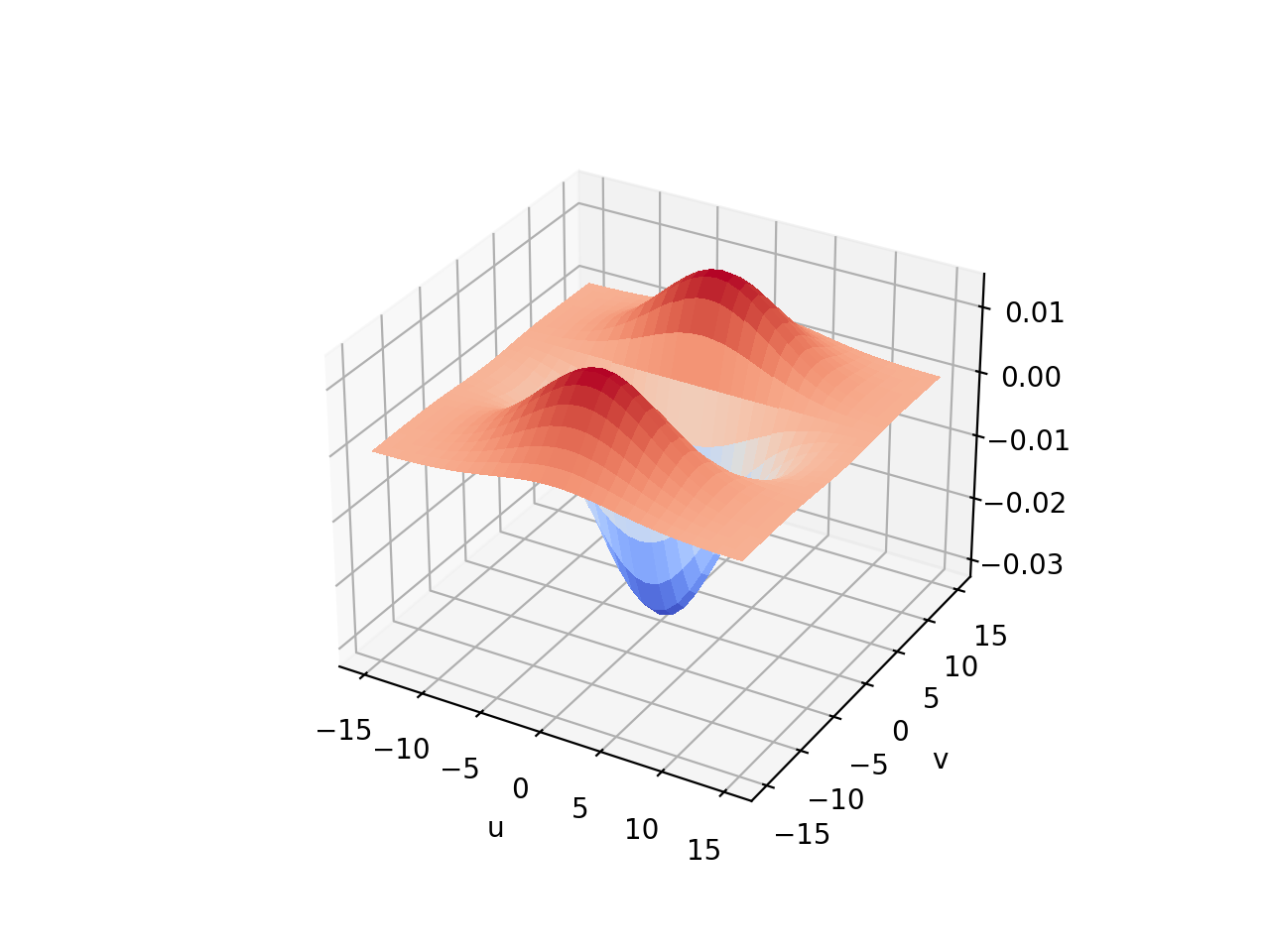
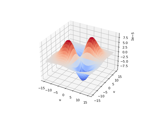
>>> Hxx, Hyy, Hxy = Kernel.HGauss(5, 15)
>>> Hxx.disp3d()
>>> Hyy.disp3d()
>>> Hxy.disp3d()

(Source code, png, hires.png, pdf)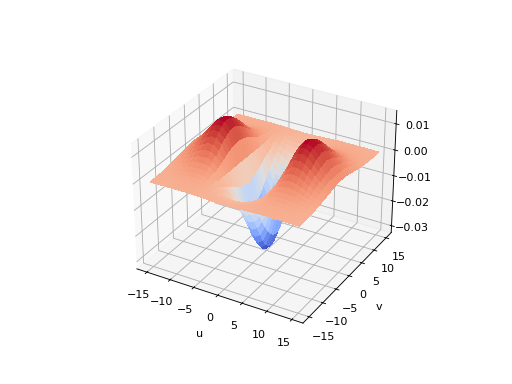

(Source code, png, hires.png, pdf)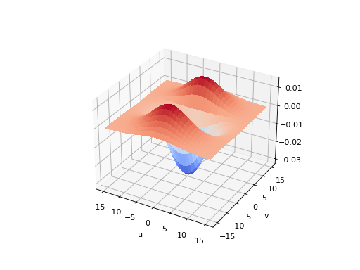

(Source code, png, hires.png, pdf)

Seealso:

DGauss Gauss Sobel