Histogram.plot

Histogram.plot(type='frequency', block=False, filled=None, stats=True, style='stack', cursor=False, alpha=0.5, title=None, log=False, samescale=False, ax=None, bar=None, **kwargs)

Plot histogram

Parameters:

• type (str, optional) – histogram type, one of: ‘frequency’ [default], ‘cdf’, ‘ncdf’

• block (bool, optional) – hold plot, defaults to False

• filled (bool, optional) – use a filled stairs plot, defaults to True for frequency plot, False for other plots

• stats (bool, optional) – draw vertical lines for mean (solid) and median (dashed), defaults to True

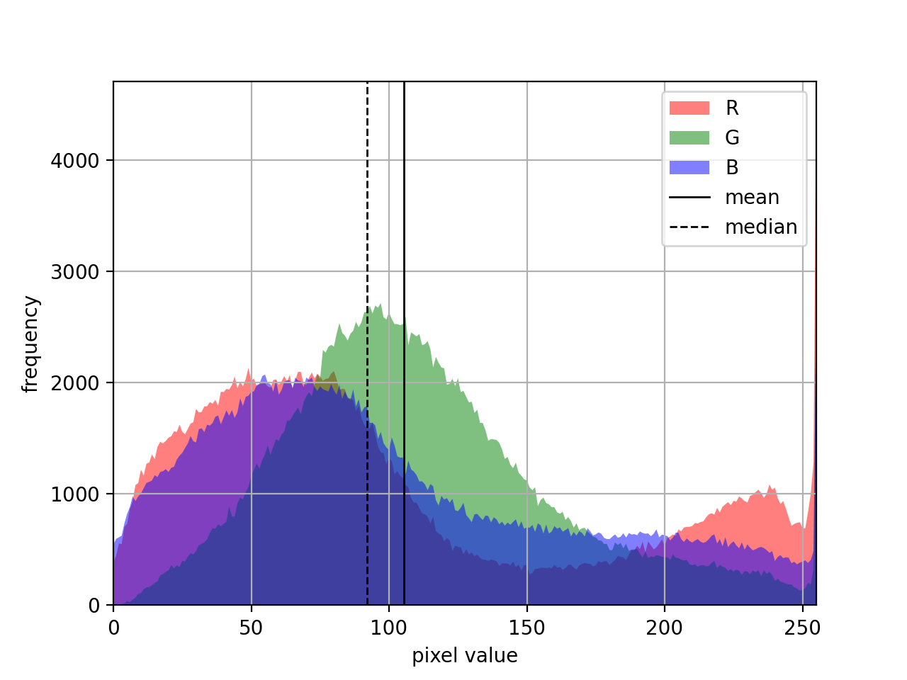
• style (str, optional) – Style for multiple plots, one of: ‘stack’ [default], ‘overlay’

• cursor (bool, optional) – enable interactive data cursor for stacked line plots, defaults to False. Cursor is ignored for overlay style.

• alpha (float, optional) – transparency for overlay plot, defaults to 0.5

• title (str, optional) – plot title, defaults to None

• log (bool, optional) – use logarithmic y-axis, defaults to False

• samescale (bool, optional) – synchronize the y-axis scale for all subplots, defaults to True

• ax (matplotlib.axes.Axes, optional) – Matplotlib axes to plot on, defaults to None (new figure)

• bar – deprecated alias for filled, use filled= instead

• kwargs – additional keyword arguments passed to Matplotlib plotting functions, plt.stairs for solid=True and plt.plot for solid=False, and plt.Polygon for style='overlay'

Raises:

• ValueError – invalid histogram type

• ValueError – cannot use overlay style for 1-channel histogram

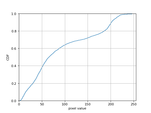
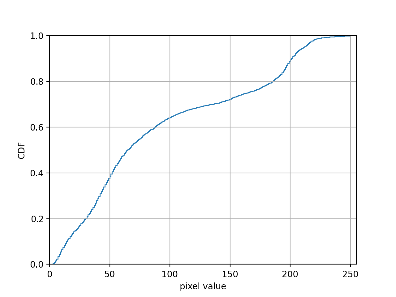
Plots the histogram using Matplotlib. For a color image, the histograms of each plane are plotted separately. The type option selects the type of histogram to plot: frequency, cdf or ncdf (normalized cumulative in the range 0 to 1).

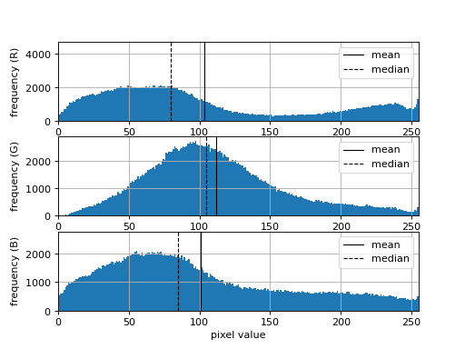
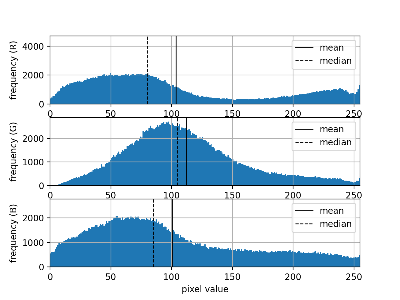
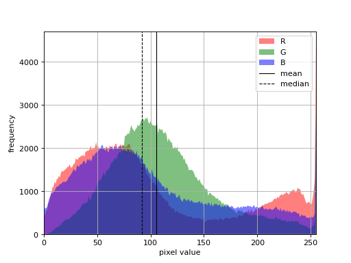
The style option selects the style for plotting multiple planes:

• stack: plot each plane in a separate subplot. The cursor option enables an interactive data cursor which displays the histogram values at the cursor position. The filled option selects whether to use a filled stairs plot.

• overlay: plot all planes in the same axes with different colors. The filled option selects whether to use a filled plot. The alpha option controls the transparency of the bars in the ‘’overlay’’ style.

samescale controls whether the y-axis scale is the same for all planes (if False, each plane is scaled independently). By default, the y-axis scale is the same for all planes, which allows for direct comparison of histogram values across planes.

The log option uses a logarithmic scale for the y-axis, which can be useful for visualizing histograms with a large dynamic range, zero values are ignored in log plots.

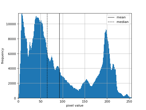
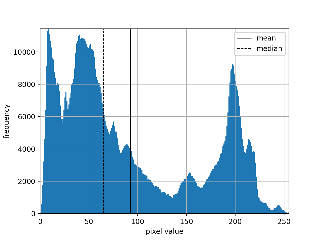
If ax is provided, the histogram is plotted on the given Matplotlib axes. For multi-plane histograms the style is overridden to ‘overlay’ since all the plots must be on one axes. If ax is not provided, a new figure and axes are created.

>>> from machinevisiontoolbox import Image
>>> im = Image.Read('street.png')
>>> hist = im.hist()
>>> print(hist)
histogram with 256 bins: xrange 0 - 255, yrange 21 - 11429
>>> hist.plot() # standard frequency plot
>>> hist.plot(type='cdf') # CDF plot

(Source code, png, hires.png, pdf)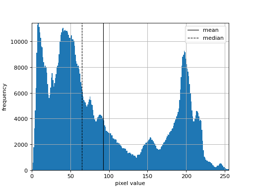

(Source code, png, hires.png, pdf)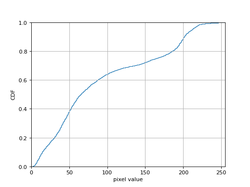

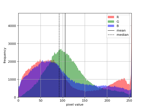
For multi-plane (color) images, the histograms of each plane can be plotted separately in stacked subplots or overlaid on the same axes.

>>> from machinevisiontoolbox import Image
>>> im = Image.Read('flowers1.png')
>>> im.hist().plot(style='stack', filled=True)
>>> im.hist().plot(style='overlay', filled=True, alpha=0.5)

(Source code, png, hires.png, pdf)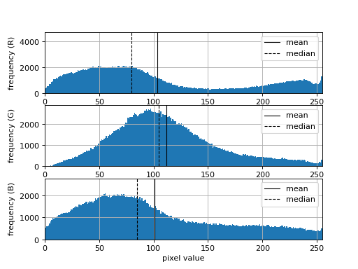

(Source code, png, hires.png, pdf)